Download
1 / 20
200 likes | 392 Views
Moment tensor inversion using observations of unknown amplification. Rosalia Daví Václav Vavryčuk. Institute of Geophysics, Academy of Sciences, Praha, Czech Republic e-mail: rosi.davi@ig.cas.cz . Green’s functions and Moment tensor. u n ( x ,t)=M pq *G np,q. (1).

E N D
Moment tensor inversion using observations of unknown amplification Rosalia Daví Václav Vavryčuk Institute of Geophysics, Academy of Sciences, Praha, Czech Republic e-mail: rosi.davi@ig.cas.cz
Green’s functions and Moment tensor un(x,t)=Mpq*Gnp,q (1) represents the n component of the displacement is the pqelement of the moment tensor • represents the spatial differentiation along the q direction of the npelementof the Green’s functions • The Green’s functionsrepresent the Earth’s response to an impulsive force acting at acertain point (source location) and propagating to the receiver location • The moment tensor represents the stresses acting on the point and describes the physical forces generated by the source.
Moment tensor inversion Misfit between calculated and observed data Solution for noise-free data Solution for noisy data
Moment tensor inversion can be performed using: High number of stations with good coverage and high signal to noise ratio are required • amplitudes • amplitude ratios • full waveforms • The inversion for waveform amplitude • linear • allows the use of several input data (P, S or P and S waves) • the convolution is reduced into multiplication (waveform is neglected) • The inversion technique is normally very sensitive to • Lack of sufficient structural information • Hypocentres location • Quantity and quality of the data un(x)=Mpq Gnp,q Focalsphere stations
Joint inversion for amplifications and moment tensor • Some waveforms can be affected by instrumental problems due to : • Wrong calibration • Wrong polarity • Site effects • The joint inversion is based on the inversion of both focal mechanims and stations amplification • It allows the use and correction of stations with amplification problems.
METHODOLOGY IT IS IMPORTANT TO HAVE HIGH VARIABILITY OF FOCAL MECHANISMS
Synthetic tests with noisy data • 3 levels of noise with 100 realizations (noise level = 0.1, 0.25, 0.50 ) • 2 main focal mechanisms with variation of 15 degrees • Different station configurations • 4 sets of events (number of events = 10, 25, 50, 100) Sparseconfiguration Denseconfiguration
Sparse configuration noise = 0.5 noise = 0.25 noise = 0.1 Number of stations with known amplification
Dense configuration noise = 0.5 noise = 0.25 noise = 0.1 number of stations with known amplification
1 known station 5 known stations Noise = 0.1 Noise = 0.50 Noise = 0.25 17 known stations 10 known stations Unknown stations
Denseconfiguration Noise = 0.50 Noise = 0.25 Noise = 0.1 station order For stations close to the nodal lines the std is high and the amplitude is small
Results from synthetic tests • Lower noise values gives lower and less scattered standard deviation • Higher number of stations with known amplifications gives smaller standard deviation • For a high variability of the focal mechanisms the results are insensitive to station locations on the focal sphere
Joint inversion with real events • We considered catalogue amplitudes of the 441 real events (Boušková et al., 2011) • 22 stations (with only one with unknown amplification – jack-knife test) • Results shows that the majority of our stations have good amplifications values • In order to confirm our results we calculated the RMS as an average of all the events at each station
WEST BOHEMIA REGION • 22 short-period seismic stations (yellow triangles) • Epicentres of the 2008 swarm (red circles) • Depth of 7.6 to 10.8 km Topographic map of the West-Bohemia/Vogtland region (from Vavryčuk, 2011)
Two principal focal mechanisms (from Vavryčuk, 2011) Most common focal mechanism (left lateral strike-slip with a strike of 169o) Second focal mechanism (right lateral strike-slip with a strike of 304o)
Tectonic structure The red lines indicate the directions of the two principal faults Their associate focal mechanisms are also shown (Vavryčuk, 2011).
LOUD and HOPD HAVE WRONG CALIBRATION ! RMS is the misfit between calculated and observed data ZHC and TRC are noisy stations
Conclusions • The joint inversion for focal mechanism and station amplifications is a poweful tool to perform moment tensor inversion • Results of the synthetic tests (with and without noisy data) show the reliability of our inversion code • Standard deviations decrease with higher number of events and stations with known amplification • Results of the inversions for real events confirm that stations with high amplifications and RMS values are affected by problems (e.g. instrumental problems such as calibration; site effects) • Stations with high RMS values but low amplifications are generally affected by problems strictly related to the inversion (e.g. noisy data or positions)
Acknowledgements We thank Josef Horálek, Alena Boušková and other colleaguesfrom the WEBNET group for providing us with the data from the 2008 swarm activity and for kind help with their preprocessing.