Download
1 / 16
160 likes | 163 Views
This lecture introduces the concepts of random processes, probability, and random variables. It covers discrete and continuous random variables, probability distributions, estimation procedures, and the interpretation of probability through relative frequencies. The lecture also discusses the center and spread of probability distributions and introduces the concepts of mean and variance.

E N D
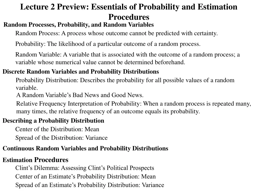
Lecture 2 Preview: Essentials of Probability and Estimation Procedures Random Processes, Probability, and Random Variables Random Process: A process whose outcome cannot be predicted with certainty. Probability: The likelihood of a particular outcome of a random process. Random Variable: A variable that is associated with the outcome of a random process; a variable whose numerical value cannot be determined beforehand. Discrete Random Variables and Probability Distributions Probability Distribution: Describes the probability for all possible values of a random variable. A Random Variable’s Bad News and Good News. Relative Frequency Interpretation of Probability: When a random process is repeated many, many times, the relative frequency of an outcome equals its probability. Describing a Probability Distribution Center of the Distribution: Mean Spread of the Distribution: Variance Continuous Random Variables and Probability Distributions Estimation Procedures Clint’s Dilemma: Assessing Clint’s Political Prospects Center of an Estimate’s Probability Distribution: Mean Spread of an Estimate’s Probability Distribution: Variance
Random Processes and Probability Random Process: A process whose outcome cannot be predicted with certainty. Tossing a coin is a random process. Drawing a card from a deck is a random process. Probability: Likelihood of a particular outcome from a random process. Consider a deck of four cards: 23 34 Experiment: Random Card Draw Shuffle the four cards thoroughly. Draw one card. Replace the card. Question: What is the probability of drawing the 2 of clubs? Answer: There is one chance in four of drawing the 2 of clubs. That is, the probability of drawing the two of clubs is ¼. Prob[2] = ¼ What is the probability of drawing the 3 of hearts? Prob[3] = ¼ What is the probability of drawing the 3 of diamonds? Prob[3] = ¼ What is the probability of drawing the 4 of hearts? Prob[4] = ¼ Random Variable: A variable that is associated with an outcome of a random process; a variable whose numerical value cannot be determined beforehand. A discrete random variable can only take on a countable number of discrete values. A continuous random variable can take on a continuous range, a continuum, of values.
Discrete Random Variables and Probability Distributions Consider a deck of four cards: 23 3 4 Prob[2] = ¼Prob[3] = ¼Prob[3] = ¼Prob[4] = ¼ Experiment: Random Card Draw Shuffle the four cards thoroughly Draw one card and record its value. Replace the card. Let v = “Value” of the selected card:2, 3, or 4. Question: What type of variable is v? Answer: v is a discrete random variable. We cannot determine the numerical value of the random variable v with certainty before the experiment is conducted. Probability Distribution of the Random Variable v Question: What do we know about the random variable v? Answer: We know how likely it is for the random variable to equal its possible values; that is, we know the probability distribution of the random variable. Card Drawn v Prob[v] 2 2 ¼ = .25 The probabilities sum to 1. 3 or 3 3 ¼ + ¼ = ½ = .50 Why? 44 ¼ = .25
A Random Variable’s Bad News and Good News Beforehand, that is, before the experiment is conducted: Bad news. We cannot determine the numerical value of the random variable with certainty. Good news. On the other hand, we can often calculate the random variable’s probability distribution telling us how likely it is for the random variable to equal each of its possible numerical values. Question: What happens if we repeat the experiment many, many times? Lab 2.1 Simulation Histogram of the Numerical Values After many, many repetitions of the experiment, v equals 2 about a quarter of the time 3 about a half of the time 4 about a quarter of the time Relative Frequency Interpretation of Probability:After many, many repetitions of the experiment, thedistribution of the actual numerical values from the experiments mirrors the random variable’s probability distribution. Question: How can we describe the general properties of a random variable; that is, how can we describe the probability distribution of a random variable? Center of its probability distribution: Mean Spread of its probability distribution: Variance
Center of the Probability Distribution : Mean (Expected Value) - The average of the numerical values after many, many repetitions of the experiment. What is the mean (expected value) of v? Card Drawn v Prob(v) After many, many repetitions of the experiment, what would v equal on average? 2 2 ¼ = .25 3 or 3 3 ¼ + ¼ = ½ = .50 2 about a quarter of the time The mean equals 3. 3 about a half of the time 44 ¼ = .25 4 about a quarter of the time For each possible value, multiply the value and its probability; then, add. Spread of the Probability Distribution : Variance - Average of the squared deviations Calculate the deviation from the mean. of thenumerical values from their mean after many, many repetitions of the experiment. Square the deviation. Multiply squared deviation by its probability. Sum the products Deviation From SquaredCard Drawn v Mean[v] Mean[v] Deviation Prob[v] 2 23 or 3 34 4 333 2 3 = 1 1 ¼ = .25½ = .50¼ = .25 3 3 = 0 0 4 3 = 1 1 For each possible value, multiply the squared deviation and its probability; then add. Lab 2.2
Continuous Random Variables and Probability Distributions Example: Dan Duffer Good News: Dan consistently drives the ball 200 yards from the tee. Bad News: His drives can land up to 40 yards to the left and up to 40 yards to the right of his target point. Dan’s target point is the center of the fairway. The fairway is 32 yards wide 200 yards from the tee. v = Lateral distance from the target point. v <0: Drive to left v > 0: Drive to right Continuous Random Variables: Can take on a continuous range, a continuum, of values. v is a continuous random variable. What does v’s probability distribution suggest? It is more likely for Dan’s drive to be close to his target than far away from it. Area Beneath Probability Distribution = + = .5 + .5 = 1.0 What does this imply?
What is the probability that Dan’s drive will land in the left rough? Prob[Drive in Left Rough] = Prob[v LessThan 16] = = .18 What is the probability that Dan’s drive will land in the lake? Prob[Drive in Lake] = Prob[v Greater Than +16] = = .18 What is the probability that Dan’s drive will land in the fairway? Prob[Drive in Fairway] = Prob[v Between 16 and +16] = .015 32 + = .015 32 + .005 32 = .020 32 = .64 Prob[Drive in Left Rough] + Prob[Drive in Lake] + Prob[Drive in Fairway] =.18+.18+.64 = 1.00 What does this imply?
Clint Ton’s Dilemma On the day before the election, Clint must decide whether or not to hold a pre-election party: If he is comfortably ahead, he will not hold the party; he will save his campaign funds for a future political endeavor (or perhaps a vacation to the Caribbean in January). If he is not comfortably ahead, he will fund a party hoping to sway some voters. There is not enough time to poll every member of the student body, however. What should he do? Econometrician’s Philosophy: If you lack the information to determine the value directly, estimate the value to the best of your ability using the information you do have. Questionnaire: Are you voting for Clint? Question: What does this suggest? Procedure: Clint selects 16 students at random and poses the question. Results: 12 students report that they will vote for Clint and 4 against Clint. This suggests that Clint leads. Estimated fraction of population supporting Clint = .75 Clint wishes to use the information collected from those polled to draw inferences about the entire population. Seventy-five percent, .75, of those polled support Clint. Dilemma: Should Clint be confident that he has the election in hand and save his resources or should he fund a party to entice more students to vote for him? Lab 2.3 Observatons: The estimated fraction, EstFrac, is a random variable. Even if we knew the actual fraction supporting Clint, ActFrac, we could not predict EstFrac before the poll. Only occasionally does the estimated fraction, EstFrac, in any one repetition of the poll equal the actual fraction. When the election is actually a toss-up, it is entirely possible that 12 (or even more) of the 16 students polled will support Clint.
Populations and Samples Question: How can sample information be used to draw inferences about the entire population? This is the question Clint must address. We begin with an unrealistic, but instructive, example. So, please be patient. Experiment: Write the names of every individual in the population on a card. Thoroughly shuffle the cards. Randomly draw one card. Ask that individual he/she supports Clint and record the answer. Replace the card.
Define v: v = 1 if the individual polled supports Clint = 0 otherwise Question: What can we say about the random variable v beforehand? Question: Can we determine with certainty the numerical value of v before the experiment is conducted? Answer: We can describe its probability distribution. Question: How can we describe a probability distribution? Answer: No. Hence, v is a random variable. Answer: Its center (mean) and spread (variance). For the moment, continue to assume that the population is split evenly; that is, suppose that half the population supports Clint and half does not: Individual’s Response v Prob[v] Center of the Probability Distribution : Mean (Expected Value): The mean (average) of the numerical values after many, many repetitions of the experiment. After many, many repetitions of the experiment, v will equal 1 about half the time 0 about half the time On average, the numerical value of v will equal ½. For each possible value, multiply the value and its probability; then add.
Individual’s Response v Prob[v] Mean[v] = Spread of the Probability Distribution : Variance. The average of the squared deviations of the numerical values from their mean after many, many repetitions of the experiment: Calculate the deviation from the mean. Square the deviation. Multiply the squared deviation by its probability Sum the products Individual’s Deviation From Squared Response v Mean[v]Mean[v] Deviation Prob[v] For Clint 1 Not for Clint 0 For each possible value, multiply the squared deviation and its probability; then, add. Lab 2.4
Generalization: p = ActFrac = Fraction of the population supporting Clint Individual’s Response v Prob[v] For Clint 1 p Not for Clint 0 1 p Center of the Probability Distribution: Mean. The mean of the numerical values after many, many repetitions of the experiment: For each possible value, multiply the value and its probability; then, add. Spread of the Probability Distribution : Variance. The average of the squared deviations of the numerical values from their mean after many, many repetitions of the experiment. Calculate the deviation from the mean. Multiply the squared deviation by its probability. Square the deviation. Sum the products. Individual’s Deviation From Squared Response v Mean[v]Mean[v] Deviation Prob[v] For Clint 1 Not for Clint 0 pp 1 p (1 p)2 p1 p 0 p = p p2 For each possible value, multiply the squared deviation and its probability; then, add. = (1 p)2 p + p2(1 p) = p(1 p)[(1 p) + p] = p(1 p) [1 p + p] = p(1 p)
Sample Size of Two Experiment: Write the names of every individual in the population on a card In the first stage: Thoroughly shuffle the cards. Randomly draw one card. Ask the first individual polled if he/she supports Clint and record the answer, v1. Replace the card. In the second stage, the procedure is repeated: Thoroughly shuffle the cards. Randomly draw one card. Ask the second individual polled if he/she supports Clint and record the answer, v2. Replace the card. Calculate the fraction of those polled supporting Clint. Estimated fraction of population supporting Clint = EstFrac EstFrac is a random variable. We cannot determine with certainty the numerical value of the estimated fraction, EstFrac, before the experiment is conducted. Question: What can we say about the random variable, EstFrac? Answer: We can describe its probability distribution. Question: How can we describe a probability distribution? Answer: Compute its center (mean) and spread (variance).
Center of the Estimated Fraction’s Probability Distribution: Mean (Expected Value). What do we know? Mean[v1] = Mean[v] = p Mean[v2] = Mean[v] = p p = ActFrac = Fraction of the population supporting Clint Arithmetic of Means: Mean[cx] = cMean[x] Mean[x+y] = Mean[x] + Mean[y] Mean[cx] = cMean[x]↓ Mean[x+y] = Mean[x] + Mean[y]↓ Mean[EstFrac] = p
Spread of the Estimated Fraction’s Probability Distribution : Variance What do we know? Var[v1] = Var[v] = p(1 p) p = ActFrac = Fraction of the population supporting Clint Var[v2] = Var[v] = p(1 p) Arithmetic of Variances: Var[cx] = c2Var[x] Var[x+y] = Var[x] + 2Cov[x, y] + Var[y] Var[cx] = c2Var[x]↓ Var[x+y] = Var[x] + 2Cov[x, y] + Var[y]↓ Question: Why are v1 and v2 independent? v1 and v2 are independent Answer: Since the card of the first name drawn is replaced, whether or not the first voter polled supports Clint does not affect the probability that the second voter will support Clint. Cov[v1,v2] = 0 In either case, the probability that the second voter will support Clint is the same; it is p, the fraction of the student body supporting Clint. Lab 2.5 Consequently, knowing the value of v1 does not help us predict the value of v2. Var[EstFrac] = More formally, knowing the value of v1 does not affect v2’s probability distribution.
Summary: Random Variables Before the experiment is conducted: Bad news. What we do not know: We cannot determine the numerical value of the random variable with certainty before the experiment is conducted. Good news. What we do know: On the other hand, we can often calculate the random variable’s probability distribution telling us how likely it is for the random variable to equal each of its possible numerical values. Relative Frequency Interpretation of Probability:After many, many repetitions of the experiment, The distribution of the numerical values from the experiments mirrors the random variable’s probability distribution. The two distributions are identical: Distribution of the Numerical Values After many, many repetitions Probability Distribution The distribution mean and variance describe the general properties of the random variable: The mean reflects the center of the distribution; more specifically, the mean equals the average of the numerical values after many, many repetitions. The variance reflects the spread of the distribution. Mean of the Numerical Values Variance of Numerical Values After many, many repetitions Mean of the Probability Distribution Variance of the Probability Distribution for One Repetition for One Repetition