Download
1 / 46
460 likes | 613 Views
Introduction to GPS radio occultation. Sean Healy (sean.healy@ecmwf.int) NWP SAF lecture, July 2, 2013. Outline. 1) Basic physics. 2) GPS (should really be “GNSS”) measurement geometry. 3) GPS radio occultation and “ Classical GPS RO retrieval ”.

E N D
Introduction to GPS radio occultation Sean Healy (sean.healy@ecmwf.int) NWP SAF lecture, July 2, 2013
Outline • 1) Basic physics. • 2) GPS (should really be “GNSS”) measurement geometry. • 3) GPS radio occultation and “Classical GPS RO retrieval”. • 4) Information content and resolution from 1D-Var. • 5) 4D-Var assimilation of GPS RO measurements (GPS RO null space). • 6) Novel applications: Planetary boundary layer information from GPS RO, • surface pressure. • 7) Ground-based GPS measurements (verybriefly). • 8) Summary and conclusions.
The basic physics – Snel’s Law (Not “Snell”, Peter Janssen) • Refractive index: Speed of an electromagnetic wave in a vacuum divided by the speed through a medium. • Snel’s Law of refraction
Measurements made using GPS signals GPS Radio Occultation (Profile information) Ground-based GPS (Column integrated water vapour) LEO GPS GPS Receiver placed on satellite GPS receiver on the ground
Radio Occultation: Some Background • Radio occultation (RO) measurements have been used by to study planetary atmospheres (Mars, Venus) since the 1960’s. Its an active technique. We simply look at how the paths of radio signals are bent by refractive index gradients in the atmosphere. • The use of RO measurements in the Earth’s atmosphere was originally proposed in 1965, but required the advent of the GPS constellation of satellites to provide a suitable source of radio signals. • Use of GPS signals discussed at the Jet Propulsion Laboratory (JPL) in late 1980’s. In 1996 the proof of concept “GPS/MET” experiment demonstrated useful temperature information could be derived from the GPS RO measurements.
GPS RO: Basic idea The GPS satellites are primarily a tool for positioning and navigationThese satellites emit radio signals at L1= 1.57542 GHz and L2=1.2276GHz (~20 cm wavelength). The GPS signal velocity is modified in the ionosphere and neutral atmosphere because the refractive index is not unity, and the path is bent because of gradients in the refractive index. GPS RO is based on analysing the bending caused by the neutral atmosphere along ray paths between a GPS satellite and a receiver placed on a low-earth-orbiting (LEO) satellite.
GPS RO geometry (Classical mechanics: Compare this picture with the deflection of a charged particle by a spherical potential!) Tangent point 20,200km α 800km a Setting occultation: as the LEO moves behind the earth we obtain a profile of bending angles, a, as a function of impact parameter, . The impact parameter is the distance of closest approach for the straight line path. Its directly analogous to angular momentum of a particle.
GPS RO characteristics • Good vertical resolution. Around 70% of the bending occurs over a ~450km section of ray-path, centred on the tangent point (point closest to surface) –it has a broad horizontal weighting function, with a ~Gaussian shape to first order! • All weather capability: not affected by cloud(?) or rain. • The bending is ~1-2 degree at the surface, falling exponentially with height. The scale-height of the decay is approximately the density scale-height. • A profile of bending angles from ~60km tangent height to the surface takes about 2 minutes. Tangent point drifts in the horizontal by ~200 km during the measurement.
Ray Optics Processing of the GPS RO Observations GPS receivers do not measure bending angle directly! The GPS receiver on the LEO satellite measures a time series of phase-delaysf(i-1), f(i), f(i+1),… at the two GPS frequencies: L1 = 1.57542 GHz L2 = 1.22760 GHz The phase delays are “calibrated” to remove special and general relativistic effects and to remove the GPS and LEO clock errors (“Differencing”, see Hajj et al. (2002), JASTP, 64, 451 – 469). Calculate Excess phase delays: remove straight line path delay, Df(i). A time series of Doppler shifts at L1 and L2 are calculated by differentiating the excess phase delays with respect to time.
LEO y r Processing of the GPS RO observations (2) The ray bending caused by gradients in the atmosphere and ionosphere modify the L1 and L2 Doppler values, but deriving the bending angles, a, from the Doppler values is an ill-posed problem (an infinite set of bending angles could produce the Doppler). The problem made well posed by assuming the impact parameter, given by (Spherical symmetry) has the same value at both the satellites. Given accurate position and velocity estimates for the satellites, and making the impact parameter assumption, the bending angle, a, and impact parameter value can be derived simultaneously from the Doppler.
The ionospheric correction We have to isolate the atmospheric component of the bending angle. The ionosphere is dispersive and so we can take a linear combination of the L1 and L2 bending angles to obtain the “corrected” bending angle. See Vorob’ev + Krasil’nikov, (1994), Phys. Atmos. Ocean, 29, 602-609. Constant given in terms of the L1 and L2 frequencies. “Corrected” bending angles How good is the correction? Does it introduce time varying biases? People are starting to think about this in the context of climate signal detection. I don’t think it’s a major problem in regions where the GPS-RO information content is largest.
The ionospheric correction: A simulated example L2 L1 Log scale The “correction” is very big!
Deriving the refractive index profiles Assuming spherical symmetry the ionospheric corrected bending angle can be written as: Corrected Bendingangle as a function of impact parameter Convenient variable (x=nr) (refractive index * radius) We can use an Abel transform to derive a refractive index profile Note the upper-limit of the integral! A priori information needed to extrapolate to infinity.
Refractivity and Pressure/temperature profiles:“Classical retrieval” The refractive index (or refractivity) is related to the pressure, temperature and vapour pressure using two experimentally determined constants (from the 1950’s and 1960’s!) This two term expression is probably the simplest formulation for refractivity, but it is widely used in GPSRO. We now use an alternative three term formulation, including non-ideal gas effects refractivity If the water vapour is negligible, the 2nd term = 0, and the refractivity is proportional to the density So we have retrieved a vertical profile of density!
“Classical” retrieval We can derive the pressure by integrating the hydrostatic equation a priori The temperature profile can then be derived with the ideal gas law: GPSMET experiment (1996): Groups from JPL and UCAR demonstrated that the retrievals agreed with co-located analyses and radiosondes to within 1K between ~5-25km. EG, See Rocken et al, 1997, JGR, 102, D25, 29849-29866.
GPS/MET Temperature Sounding (Kursinski et al, 1996, Science, 271, 1107-1110, Fig2a) GPS/MET - thick solid. Radiosonde – thin solid. Dotted - ECMWF anal. Results like this by JPL and UCAR in mid 1990’s got the subject moving. (Location 69N, 83W. 01.33 UT, 5th May, 1995)
Limitations of classical retrieval: we can’t neglect water vapour in the troposphere! Difference between the lines show the impact of water vapour. Simulated ignoring water vapour
GPSRO limitations – upper stratosphere In order to derive refractivity the (noisy – e.g. residual ionospheric noise) bending angle profiles must be extrapolated to infinity – i.e., we have to introduce a-priori. This blending of the observed and simulated bending angles is called “statistical optimisation”. The refractivity profiles above ~35 km are sensitive to the choice of a priori. The temperature profiles require a-priori information to initialise the hydrostatic integration. Sometimes ECMWF temperature at 45km! I would be sceptical about any GPSRO temperature profile above ~35-40 km, derived with the classical approach. It will be very sensitive to the a-priori!
Limitations – lower troposphere • The refractivity profiles in the lower troposphere are biased low when compared to NWP models, particularly in the tropics. See Ao et al JGR, (2003), 108, doi10.1029/2002JD003216. • Atmospheric Multipath processing – more than one ray is measured by the receiver at a given time: • Wave optics retrievals: Full Spectral Inversion. Jensen et al • 2003, Radio Science, 38, 10.1029/2002RS002763. (Also improve vertical. res.) • Improved GPS receiver software: Open-loop processing. Single ray region – ray optics approach ok! Multipath: More than one ray arrives at the receiver. They interfere.
Physical limitations in lower troposphere Atmospheric defocusing: If the bending angle changes rapidly with height, the signal reaching the receiver has less power A tube of rays is spread out by the ray bending and the signal to noisefalls. Atmospheric ducting: if the refractive index gradient exceeds a critical value the signal is lost Not affected by clouds?But we often get ducting conditions near the top of stratocumulus clouds
Maximum bending angle value(related to defocusing) Seems obvious but the receiver has to be measuring a long time to see the large bending angle values. We rarely see an observed bending above ~0.05 rads.
Data availability • The “proof of concept” GPS/MET mission in 1996 was a major success. This led to a number of missions of opportunity, proposals for a constellation of LEO satellites and first dedicated operational instruments. • Current status: • Missions of opportunity: GRACE-A, TerraSAR-X, C/NOFS. • The COSMIC constellation of 5 LEO satellites was launched 2006. Currently providing ~1400 occultations per day (2200 at peak). • The GRAS instrument on METOP-A and METOP-B provides ~1300 measurements. GRAS is the only fully operational instrument. GRAS on METOP-B has been assimilated since May 21, 2013.
But why are GPS RO useful for NWP given that we already have millions of radiance measurements? 1) GPS RO can be assimilated without bias correction*. They are good for highlighting model errors/biases. Most other satellite observations require bias correction to the model. GPSRO measurements anchor the bias correction of radiance measurements. Importance of anchor measurements in weak constraint 4D-Var. (Climate/reanalysis applications). 2) GPS RO (limb sounders in general) have sharper weighting functions in the vertical and therefore have good vertical resolution properties. The GPSRO measurements can “see” vertical structures that are in the “null space” of the satellite radiances. *The observed refractivity values are biased low near the surface. See Ao et al, JGR, 2003, D18, 4577, doi:10.1029/2002JD003216.
Use of GPS RO in NWP • Most NWP centres assimilate either bending angle or refractivity. • The classical retrieval is very useful for understanding the basic physics of the measurement, but not recommended for use in NWP. • We can test bending angle and refractivity observation operators in 1D-Var retrievals to estimate the information content and vertical resolution of the measurements.
1D-Var retrieval The 1D-Var retrieval minimises the cost function: The observation operator - simulating bending angles or refractivity from the forecast state. The 1D-Var approach provides a framework for testing observation operators that we might use in 3D/4D-Var assimilation. We can also investigate various information content measures.
1D bending angle weighting function (Normalised with the peak value) Weighting function peaks at the pressure levels above and below the ray tangent point. Bending related to vertical gradient of refractivity: Sharp structure near the tangent point Increase the T on the lower level – reduce the N gradient – less bending! Increase the T on the upper level – increase N gradient more bending! hydrostatic tail (See also Eyre, ECMWF Tech Memo. 199.) Very sharp weighting function in the vertical – we can resolve structures that nadir sounders cannot!
Useful 1D-Var diagnostics Linearised forward model Solution error cov. matrix • 1D-Var provides an estimate of the solution error covariance matrix. • Information content: related to the uncertainty before and after the measurement is made. • It also gives vertical resolution diagnostics – the averaging kernel. Assumed observation error cov. matrix Assumed background error cov. Matrix.
1D-Var information content (Collard+Healy, 2003)QJRMS, 2003, v129, 2741-2760 RO provides good temperature information between 300-50hPa. IASI retrieval performed with 1000 channels, RO has 120 refractivity values. (Refractivity errors are vertically correlated because of the Abel transform). In theory RO should provide useful humidity information in the troposphere.Further work needed to demonstrate the value of water vapour derived from GPSRO at NWP centres. RO provides very little humidity information above 400hPa. The “wet” refractivity is small compared to the assumed observation error.
Vertical resolution (1D-Var averaging kernels – how well a retrieval can reproduce a spike)
Assimilation at ECMWF • We assimilate bending angles with a 1D operator. We ignore the 2D nature of the measurement and integrate • The forward model is quite simple: • evaluate geopotential heights of model levels • convert geopotential height to geometric height and radius values • evaluate the refractivity, N, on model levels from P,T and Q. • Integrate, assuming refractivity varies exponentially between model levels. (Solution in terms of the Gaussian error function). • We now include tangent point drift (May 2011). • 2D operator being tested currently at ECMWF. Convenient variable (x=nr) (refractive index * radius)
Impact on ECMWF operational analyses • We would expect improvements in the stratospheric temperatures. The fit to radiosonde temperatures is improved (eg, 100 hPa, SH). GPSRO used in operations since 12th December, 2006.
Mean analysis/increments over Antarctica for Feb. 2007 Mean analysis Mean temperature increment Black = GPSRO included Red = No GPSRO measurements assimilated GPSROcorrecting errors in the null-space of radiance measurements! But GPSRO also has a null-space!
GPS RO also has a “null space” • The measurement is related to density (~P/T) on height levels and this ambiguity means that the effect of some temperature perturbations can’t be measured. Assume two levels separated by z, with temperature variation T(z) between them. Now add positive perturbation ΔT(z)~exp(z/H),where H is the density scale height • The density as a function of height is almost unchanged. A priori information required to distinguish between these temperature profiles. This is the GPS-RO null space. P and T have increased at z, but the P/T is the same. Pu,Tu,(P/T)u T(z)+ΔT(z) z2=z+Δz z, T(z) z P,T,P/T
Null space – how does a temperature perturbation propagate through the bending angle observation operator 1K at ~25km Assumed ob errors The null space arises because the measurements are sensitive to density as function of height (~P(z)/T(z)). A priori information is required to split this into T(z) and P(z). We can define a temperature perturbation ΔT(z)~exp(z/H) which is in the GPSRO null space. Therefore, if the model background contains a bias of this form, the measurement can’t see or correct it.
Novel applications: Deriving planetary boundary layer information from GPSRO measurement • Some papers have suggested that we should be able to derive information on the height of the planetary boundary layer from the GPSRO bending angle and refractivity profiles. • Sokolovskiy et al, 2007, GRL, 34,L18802,doi10.1029/2007GL030458 • VonEngeln et al, 2005, GRL, 32, L06815,doi10.1029/2004GL022168 • The central idea is that you see big changes in the bending angle and refractivity profile gradient across the top of the PBL.
Sokolovskiy et al, (2007) It is a very interesting idea, which still needs to be investigated further. Horizontal gradient errors. Meaning of PBL height averaged over 300-400 km?
Observed and first-guess bending angle from operations (2008.08.29) 22:59, lat=-11, lon=-157 Solid line = simulated Dot-dash = observed We don’t seem to be seeing these really sharp structures in the observations. Atmospheric defocusing? SNR drops so we can’t measure the really sharp structure.
Surface pressure information from GPS-RO • Measuring or retrieving surface pressure information from satellite radiances has been discussed for many years (Smith et al, 1972). • The GPS-RO measurements have a sensitivity to surface pressure because they are given as a function of height. • Hydrostatic integration is part of the GPS-RO forward model. If we increase the surface pressure the bending angle values increase. • Can GPS-RO constrain the surface pressure analysis when all conventional surface pressure measurements are removed?
NH 12 hour PMSL forecast scores Mean GPS-RO included. The GPS-RO measurements manage to stabilise the bias. Standard deviation
Ground-based GPS measurements • ECMWF currently monitors ground based GPS zenith delay measurements in operations. GPS Consider a receiver placed on the surface. Ignoring bending, the excess slant delay caused by the atmosphere is The slant delays are mapped to a zenith delays using mapping functions. (eg Niell, 1996, J. Geophys. Res., 101(B2), 3227-3246) z Straightline path
ECMWF monitors zenith total delay Typically 2.3 m “Hydrostatic delay” “wet delay” Information content The “hydrostatic delay” is large (90% of total), but it is only really sensitive to the surface pressure value at the receiver. The “wet delay” is smaller, but more variable. The wet delay is related to the vertical integral of the water vapour density. (See Bevis et al, (1992), JGR, vol. 97, 15,787-15,801, for the classical retrieval of integrated water vapour. )
Summary • GPS RO is a satellite-to-satellite limb measurement. • Outlined the basic physics of the GPS RO technique and the classical retrieval. • Measurements do not require bias correction. This may be important for climate applications. The observation operators are quite simple. Very good vertical resolution, but poor horizontal resolution (~450 km average). Also, be wary of classical temperature retrievals above 35-40 km. They mainly contain a-priori information. • Information content studies suggest GPS RO should provide good temperature information in the upper troposphere and lower/mid stratosphere. Operational assimilation of GPSRO supports this. • New applications: PBL work is an interesting application, but more work required. Surface pressure information from GPS-RO. • Briefly outlined the ground-based GPS technique for estimating integrated water vapour.
Useful GPSRO web-sites • International Radio Occultation Working Group (IROWG) www.irowg.org. • The COSMIC homepage www.cosmic.ucar.edu. This contains latest information on the status of COSMIC and an extensive list of papers www.cosmic.ucar.edu/references.html, with some links to .pdfs of the papers, workshops. • The Radio Occultation Meteorology (ROM) SAF homepage www.romsaf.org. • You can find lists of ROM SAF publications www.romsaf.org/publications. • Links to GPS RO monitoring pages (Data quality, data flow of COSMIC, GRACE-A, CHAMP and GRAS). • In addition, you can register and download for the ROM SAF’s Radio Occultation Processing Package (ROPP). This F90 software package containing pre-processing software modules,1D-Var minimization code, bending angle and refractivity observation operators and their tangent-linears and adjoints. • 2008 ECMWF/GRAS SAF Workshop papers and presentations. • www.ecmwf.int/newsevents/meetings/workshops/2008/GPS_radio_occultation/ • index.html