Download
1 / 19
190 likes | 375 Views
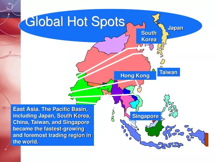
Global Hot Spots. Japan. South Korea. Taiwan. Hong Kong. East Asia. The Pacific Basin, including Japan, South Korea, China, Taiwan, and Singapore became the fastest-growing and foremost trading region in the world. Singapore. Figure 9.1.

E N D
Global Hot Spots Japan South Korea Taiwan Hong Kong East Asia. The Pacific Basin, including Japan, South Korea, China, Taiwan, and Singapore became the fastest-growing and foremost trading region in the world. Singapore Figure 9.1
NAFTA. The North American Free Trade Agreement makes trade easier between Canada, Mexico, and the United States. Other Latin American countries may follow suit. U.S. Sunbelt.The sunbelt is attracting many firms normally entrenched in the industrial heartland of the United States owing to lower labor costs, less unionism, and a more-attractive climate. Mexico. Thousands of plants have been built by firms across the world in the maquiladoras on Mexico's northern boarder. Figure 9.1
Europe. The European Union (EU) encompasses 15 member nations and special arrangements with most other European states. Figure 9.1
Former Communist Countries. The population of 410 million promises huge market opportunities and attractive possibilities for joint ventures. Russia Figure 9.1
Managing Global Operations • Other Languages • Different Norms and Customs • Workforce Management • Unfamiliar Laws and Regulations • Unexpected Cost Mix
Location Decisions - Manufacturing • Favorable Labor Climate • Proximity to Markets • Quality of Life • Proximity to Suppliers • Proximity to Parent Company • Utilities, Taxes, and Real Estate Costs
Location Decisions - Services • Proximity to Customers • Transportation Costs and Proximity to Markets • Location of Competitors • Site-Specific Factors
Erie North Scranton State College Pittsburgh Harrisburg Philadelphia Uniontown Location WS = (25 x 4) + (20 x 3) + (20 x 3) + (15 x 4) + (10 x 1) + (10 x 5) WS = 340 Location Factor Weight Score Total patient miles per month 25 4 Facility utilization 20 3 Average time per emergency trip 20 3 Expressway accessibility 15 4 Land and construction costs 10 1 Employee preference 10 5
Location North 200 Erie A (50, 185) 150 Scranton State College B (175, 100) y(miles) 100 Pittsburgh Harrisburg Philadelphia 50 Uniontown 0 50 100 150 200 250 300 x (miles) East
dAB=( xA – xB )2 + (yA – yB )2 Location Euclidean distance dAB= (50 – 175)2 + (185 – 100)2 dAB= 151.2 miles
Location Rectilinear distance dAB=| xA – xB | + |yA – yB | dAB=| 50 – 175 | + | 185 – 100 | dAB= 210 miles
Tutor 9.2 - Distance Measures Enter the x and y coordinates of the two towns. xy Erie (Point A) 50 185 State College (Point B) 175 100 To find the Euclidian distance, subtract the second town’s x value from that of the first town, and square the result. Do the same with the two y values. Then add the two and compute the square root. (Erie x – State College x)2 15.625 Euclidian distance 151.16 (Erie y – State College y)2 7,225 To find the rectilinear distance, get the absolute value of the result of subtracting the second town’s x from the first town’s. Do the same with y. Then add the absolute distances together. (Erie x – State College x) 125 Rectilinear distance 210 (Erie y – State College y) 85 Using OM Explorer
North 6 (5.5, 4.5) [10] E 5 C A (8, 5) [10] (2.5, 4.5) 4 [2] 3 B G y(miles) F D (2.5, 2.5) (9, 2.5) 2 [5] (5, 2) [14] (7, 2) [7] [20] 1 0 1 2 3 4 5 6 7 8 9 10 x (miles) East Location (a) Locate at C (5.5, 4.5) Census Population Distance Tract (x, y) (l) (d) ld A (2.5, 4.5) 2 3 + 0 = 3 6 E (8, 5) 10 2.5 + 0.5 = 3 30
6 5 4 3 y(miles) 2 1 0 1 2 3 4 5 6 7 8 9 10 x (miles) East Location (a) Locate at C (5.5, 4.5) North (5.5, 4.5) Tract ld A 6 B 25 C 0 D 21 E 30 F 80 G 77 Total 239 [10] E C A (8, 5) [10] (2.5, 4.5) [2] B G F D (2.5, 2.5) (9, 2.5) [5] (5, 2) [14] (7, 2) [7] [20]
1 2 3 4 5 6 7 8 9 10 x (miles) East Location (b) Locate at F (7, 2) North (5.5, 4.5) Tract ld A 14 B 25 C 40 D 14 E 40 F 0 G 35 Total 168 [10] E C A (8, 5) [10] (2.5, 4.5) [2] B G F D (2.5, 2.5) (9, 2.5) [5] (5, 2) [14] (7, 2) [7] [20]
6 5 4 3 y(miles) 2 1 0 1 2 3 4 5 6 7 8 9 10 x (miles) East Location Alternative Locations North 391 283 233 253 355 247 197 233 331 223 173 326 228 218 168
North 6 (5.5, 4.5) [10] E 5 C A (8, 5) [10] (2.5, 4.5) 4 Census Population Tract (x, y) (l) lxly A (2.5, 4.5) 2 5 9 B (2.5, 2.5) 5 12.5 12.5 C (5.5, 4.5) 10 55 45 D (5, 2) 7 35 14 E (8, 5) 10 80 50 F (7, 2) 20 140 40 G (9, 2.5) 14 126 35 Totals 68 453.5 205.5 [2] 3 y(miles) B G F D (2.5, 2.5) (9, 2.5) 2 [5] (5, 2) [14] (7, 2) [7] [20] 1 0 1 2 3 4 5 6 7 8 9 10 x (miles) East Location Center of Gravity Approach
453.5 68 205.5 68 Location Center of Gravity Approach x* = 6.67 y* = 3.02 x* = y* =
Location Center of Gravity Approach