Download
1 / 43
430 likes | 518 Views
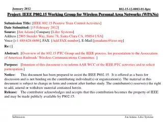
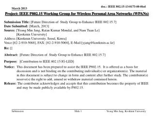
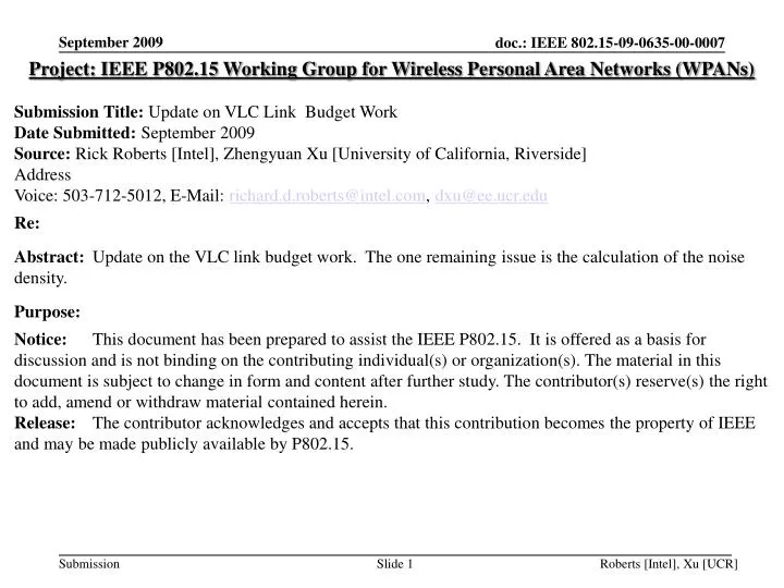
Project: IEEE P802.15 Working Group for Wireless Personal Area Networks (WPANs) Submission Title: Update on VLC Link Budget Work Date Submitted: September 2009 Source: Rick Roberts [Intel], Zhengyuan Xu [University of California, Riverside] Address

E N D
Project: IEEE P802.15 Working Group for Wireless Personal Area Networks (WPANs) Submission Title: Update on VLC Link Budget Work Date Submitted: September 2009 Source: Rick Roberts [Intel], Zhengyuan Xu [University of California, Riverside] Address Voice: 503-712-5012, E-Mail: richard.d.roberts@intel.com, dxu@ee.ucr.edu Re: Abstract: Update on the VLC link budget work. The one remaining issue is the calculation of the noise density. Purpose: Notice: This document has been prepared to assist the IEEE P802.15. It is offered as a basis for discussion and is not binding on the contributing individual(s) or organization(s). The material in this document is subject to change in form and content after further study. The contributor(s) reserve(s) the right to add, amend or withdraw material contained herein. Release: The contributor acknowledges and accepts that this contribution becomes the property of IEEE and may be made publicly available by P802.15. Roberts [Intel], Xu [UCR]
VLC Link Budget Roberts [Intel], Xu [UCR]
Outline Relation between radiometric and photometric parameters Ascertaining the LED parameters of interest Path loss due to light propagation Received optical and electrical power Receiver noise density An example based on vendor data Roberts [Intel], Xu [UCR]
Radiometric (Physical) vs. Photometric (Visual) Roberts [Intel], Xu [UCR]
The human eye and the detector diode have different frequency responses and hence perceive the same LED source differently. A white LED spews optical power across a range of wavelengths (mW/Hz) LED Detector Diode Eyeball Roberts [Intel], Xu [UCR]
Units For data link budgets we want to use Radiometric units For illumination applications we want to use Photometric units (which include the frequency response of the human eye) LED vendors generally only provide Photometric data since illumination is the market today and the use of LEDs for data is an obscure usage. Roberts [Intel], Xu [UCR]
Ascertaining the LED parameters of interest On the following pages, equation (2.2.1) and Figure 2.1.1 are from the book Introduction to Solid-State Lighting by A. Zukauskas, et.al. The equation relates the power spectral distribution S() (W/nm) to luminous flux v (lm). Roberts [Intel], Xu [UCR]
Find transmitted power and spectral density The LED total luminous flux Ft (lumens) is given as (2.2.1) V() is the relative luminous efficiency function defined by CIE and given in the table (from internet) and curve (from the book Fig 2.1.1) Fig 2.1.1 Sometimes it is convenient to use a Gaussian curve fitting for V() (from internet) Roberts [Intel], Xu [UCR]
Warm White Neutral White Cool White H L Typically we only know a normalized spectral curve St’() instead of St() in (2.2.1). Denote their relation as St()=ct St’() with an unknown scaling factor ctthat can be found from Remark: The above step to find St() can be skipped if St() can be either measured using a spectrometer or supplied by the LED vendor. Roberts [Intel], Xu [UCR]
Find transmitter luminous spatial intensity distribution I0 gt() A normalized spatial luminous intensity distribution gt() is provided by a vendor. We need to find the axial intensity I0 that is defined as the luminous intensity (candelas) on the axis of the source (zero solid angle). Since the luminous flux Ft is also a spatial integral of spatial luminous intensity in addition to spectral integral we used before, we have the following relation where max and max are the source beam solid angle and maximum half angle respectively and max=2(1-cosmax). Note: if the axial intensity is provided by the vendor then one only need convert the intensity from candelas to watts/sr. normalized spatial luminous intensity distribution Roberts [Intel], Xu [UCR]
Path loss due to line-of-sight (LOS) light propagation Roberts [Intel], Xu [UCR]
LOS Link Model • The receiver distance to the source is D • The receiver aperture radius is r and receiver area is Ar • The angle between receiver normal and source-receiver line is • The angle between source beam axis and source-receiver line (viewing angle) is • The solid angle of the receiver seen by the source is r Roberts [Intel], Xu [UCR]
The luminous angular intensity of the source at the receiver direction is I0gt(), and therefore the receiver ingested luminous flux Fr=I0gt()r. The luminous path loss can be represented as where r is the receiver solid angle which satisfies Arcos()D2r . Power path loss Lp can be proven equal to luminous path loss LL as follows: • Optical power can be written as • In LOS free space propagation, path loss is assumed independent of wavelength. Power path loss can be represented as Lp=S2()/S1()=P2/P1. • Luminous flux is related to S()as , which is linear with S() • Therefore, LL=F2/F1=Lp. Roberts [Intel], Xu [UCR]
f where Sr() is the received light power spectral density (W/nm) Rr() is the receiver filter spectral response RD() is the detector responsivity (A/W at ) f Find received optical and electrical power Now that we have known the optical power loss due to LOS propagation, we can obtain the received optical spectral density from transmitter optical spectral density as Received optical power Suppose we use a photodiode detector to receive the signal light. We can obtain the electrical power of the signal as The detector diode vendors are giving us the info we need Roberts [Intel], Xu [UCR]
Exemplary Optical Filter Response ideal typical http://www.newport.com/images/webclickthru-EN/images/2226.gif Roberts [Intel], Xu [UCR]
Summary of key steps to obtain received optical power and electrical power • Calculate transmitter (source) optical power from given luminous flux Ft (lumens) and normalized spectral curve St’() • Find the transmitter axial intensity I0 from given luminous flux Ftand luminous spatial intensity distribution gt() • Find receiver ingested luminous flux Fr from receiver solid angle and transmitter luminous spatial intensity distributionI0 gt() • Find the luminous path loss LLfrom Ft and Fr • Prove power path loss Lp is equal to luminous path loss LLfrom which to find received optical power spectral curve Sr() • Calculate received optical power and electrical power Roberts [Intel], Xu [UCR]
Comment on RX aperture vs. magnification factor It is the author’s opinion that the RX aperture determines the “brightness” of an observed object and that the field of view determines the magnification factor of an observed object. That is, for a given aperture the magnification factor determines how big an object appears but not how bright an object appears. The observed brightness is solely a function of the aperture size. It should be noted that the field of view, and hence the magnification factor, is a function of the focal distance. Long focal distance Short focal distance Same aperture lens Roberts [Intel], Xu [UCR]
Receiver Noise Density Roberts [Intel], Xu [UCR]
Determining the noise density No • What are the sources that contribute to the noise density? • Photodetector Noise • Transimpedance Amplifier Noise • Ambient “in-band” noise • Out-of-band cross modulation noise due to photodetector non-linearity • Others? Nambient Ntransamp NOOB Ndiode Modulation Domain Spectrum Analyzer Signal Of Interest (SOI) SOI Non-linear noise bleed over Out-of-Band (OOB) Interference Signal Ambient Noise Floor Modulation Domain Spectrum Roberts [Intel], Xu [UCR]
Ambient “In-Band” Noise Floor This probably has to be empirically measured for many different environments Roberts [Intel], Xu [UCR]
Cross-modulation of Out-of-Band noise from other VLC signals into the SOI ignore? Roberts [Intel], Xu [UCR]
CL R2 The detector itself contributes a noise density Ndiode (W/ Hz) (A/ Hz) detector model C2 R2 q is the electron charge (1.6e-19 coulombs) ID is the dark current IS is the signal current IB is the background light induced current B is the bandwidth (B=1 Hz for N0) k is Boltzmann’s constant (1.38e-23 J/K) T is the Kelvin temperature (~290 K) RSH is the shunt resistance Roberts [Intel], Xu [UCR]
TI OPA111 R2=10e6 ohms Transimpedance Amplifier Noise Analysis Ref. TI/Burr-Brown Application Bulletin SBOA060 “Noise Anaysis of FET Transimpedance Amplifiers” Assume R3=0 http://focus.ti.com/lit/an/sboa060/sboa060.pdf Roberts [Intel], Xu [UCR]
TI OPA111 The resistors and capacitors form critical corner frequencies as shown below: Roberts [Intel], Xu [UCR]
Noise Regions for the TI OPA228 Typically op-amps have three noise regions … the above noise regions are for the TI OPA111 op-amp. It is anticipated most outdoor VLC implementations will be bandpass systems operating in noise region 3. Roberts [Intel], Xu [UCR]
The approximation output noise is given by where Roberts [Intel], Xu [UCR]
The signal current is given as Then electrical SNR is used in numerical example later on Roberts [Intel], Xu [UCR]
Eb/No Dimensional Analysis Roberts [Intel], Xu [UCR]
An example based upon vendor data Roberts [Intel], Xu [UCR]
Example OSRAM white LED: LUW W5SM-JYKY-4P7R-Z Used parameters in red box Roberts [Intel], Xu [UCR]
Normalized radiant power spectrum density Roberts [Intel], Xu [UCR]
Normalized spatial luminous intensity distribution Roberts [Intel], Xu [UCR]
Thorlabs High Speed Detector: FDS010 PIN Silicon Diode Roberts [Intel], Xu [UCR]
optical filter band 430nm ~ 470nm An example responsivity curve (A/W) FDS-010 http://www.thorlabs.de/Thorcat/0600/0636-S01.pdf Roberts [Intel], Xu [UCR]
Thorlabs filter response Roberts [Intel], Xu [UCR]
Parameters Slide 36 Roberts [Intel], Xu [UCR]
Results Roberts [Intel], Xu [UCR]
Companion Xcel Spreadsheet Analysis Under Development Roberts [Intel], Xu [UCR]
Link Budget Spreadsheet Results Under Development Roberts [Intel], Xu [UCR]
Backup Slides Roberts [Intel], Xu [UCR]
LED Spectrum (white LED) Flux / bandwidth (W/nm) The detector diode vendors are giving us the info we need This is the information we need from the LED vendor For best performance we want the detector spectral responsivity to be “matched” to the LED spectral density. In general this is hard to due, especially for white LEDs. Where T() is the transmitter power spectral density (W/nm) R() is the detector responsivity (A/W at ) L() is the propagation loss (loss at ) Roberts [Intel], Xu [UCR]