Download
1 / 57
570 likes | 738 Views
Stability Analysis of a Complete RTL-to GDS2 Design Flow. Howard A. Landman. Introduction.

E N D
Stability Analysis of a Complete RTL-to GDS2 Design Flow Howard A. Landman
Introduction • This is a written version of a web seminar that I gave for Magma Design Automation on April 30, 2003. Since there is no voice-over, this version contains more detail. It also has more data points for both test cases. • You can see the original web seminar at http://webevents.broadcast.com/cmp/wcs/detail.asp?event_id=5877
Outline • Purpose & Methodology • Results • Test Case A - control logic • Test Case B - CPU core • Conclusions
Purpose • This study looked at the stability or predictability of Magma's complete RTL to layout flow (Blast RTL + Blast Fusion). • To do this, I reused and extended techniques that I used earlier on synthesis tools.
Previous studies • In SNUG 1998 I presented a similar study of Synopsys Design Compiler called Visualizing the Behavior of Logic Synthesis Algorithms. (Available on deepchip and elsewhere.) It explains the methodology in detail and even includes code fragments. • Ambit BuildGates studied but not published
Conclusions from synthesis studies • EDA tools may behave randomly as inputs vary slightly • Randomness can be measured and quantified if many runs are done • Degree of randomness is a useful quality metric for tools (less randomness is better)
Methodology • Vary delay constraints while keeping RTL etc. constant • Record input Constraint and output Delay and Area • Plot • D as function of C • A as function of C • D vs A (banana curve)
Methodology (continued) • The basic idea is to test the stability of a tool or design flow by slightly varying one of its input parameters, and looking at how the outputs change. • Here we vary the delay constraints (desired clock period), but other choices are also possible.
Why should you care? • Want design flow to give predictably good results and not vary wildly every time you tweak something. • Otherwise • Cannot be sure whether small problems are real or result of tool fluctuation • May have to iterate to get good result
Stability != Goodness • Stability is not the same as goodness. • A tool could reliably give bad results; it would then be stable but not good. • However, a very good tool must be stable, or its randomness will prevent it from finding the best solution much of the time.
Current Study (1) • Magma asked me to perform a stability analysis for their tools - and broadcast the results - before they even knew what I would say! • In an industry that's typically cautious or even fearful of anything like a benchmark, it's highly commendable for a company to be this open.
Aside on Benchmarks • Some people might be tempted to treat this study as a comparative benchmark of Magma vs. Synopsys. This would be utterly wrong for so many reasons that it would take several foils to list them all. No comparable study of the latest and greatest Synopsys tools has been published. (But it would be interesting to see one, would it not?)
Current Study (2) • Same kind of analysis, but for a complete RTL to layout flow - Magma BlastRTL and BlastFusion (internal red build of 3.2) • Synthesis-only results are not as interesting as they used to be - we care about the whole flow • Physical effects now dominate • RTL-to-GDS flows are maturing • Tools are fast enough to allow many runs on small to medium modules
Current Study (3) • Included automated steps like: • scan insertion, stitching, reordering • clock tree, hold time fixes, ''useful skew'' • spare cells • Left out manual steps (e.g. DRC fixes) • Also left out xtalk / signal integrity steps • As before, plot relations between constraint, delay, and area.
Current Study (4) • Flow broken into 3 steps • Step 0: Read RTL • Step 1: Apply constraints, synthesize • Step 2: Load floorplan, place and route • Step 0 run only once (takes 1-3 minutes) • Run times given are for steps 1 and 2 combined on a 2.4 GHz Linux blade
Test Case A • Staging control logic from a microprocessor • 4.7 K to 9.1 K cells in .13 um TSMC library • 1.7 to 3.6 nS cycle time • 3 layer metal (metal 2 most difficult) • Floorplan scaled with cell area (roughly constant utilization) • Flow includes spare cell insertion • Runtime 7 to 18 minutes
Plot 1: Delay vs. Constraint • Plots clock period of final laid-out design as a function of the clock period requested in the constraints. • Pink line is where delay = constraint. Below right of line is meeting timing and above left is missing timing.
Delay is somewhat unpredictable in this range, but we don’t care because we’re meeting timing with a lot of margin.
Delay is somewhat unpredictable in this range, but we don’t care because we’re meeting timing with a lot of margin. It’s more stable when timing gets hard to meet. Let’s look at a blowup of that range ...
Peak-to-peak delay variation about 10% ... … but standard deviation much less. Most results are close to optimal.
Plot 2: Area vs. Constraint • Plots cell area of final laid-out design as a function of the clock period requested in the constraints. • Fastest result had area 1.02 sq. mm. Any area above that is wasted.
Overconstraining the tools causes area to increase with no benefit in speed (area of fastest result)
Peak-to-peak area variation: about 7% but only when severely overconstrained
Peak-to-peak area variation: about 7% but only when severely overconstrained Less under achievable constraints
Plot 3: Area vs. Delay • Sometimes called ''Banana Curve'' • Plots cell area of final laid-out design vs. its delay. • Shows achievable tradeoff between delay and area.
In this region, spending more area doesn’t buy anything in delay!
In this region, can reduce delay at essentially zero cost in area
Conclusions A • Severely overconstraining BlastRTL / BlastFusion is a bad idea! • Area gets worse, run time gets worse • Timing does not get better! • Why? I can speculate … • Working on Total Negative Slack? • No ''critical range'' limit? • Best to tell the tool the truth
Test Case B • CPU core with bus and memory interfaces • Multiple clocks & resets, JTAG, BIST, PLL • 22.3 K to 41.3 K cells • 3.8 to 7.0 nS cycle in NEC 0.10 um library • 6 layer metal • Fixed floorplan, not scaled • Includes scan insertion / stitching / reordering • Runtime 54 to 110 minutes
Plot 1: Delay vs. Constraint • Plots clock period of final laid-out design as a function of the clock period requested in the constraints. • Pink line is where delay = constraint. Below right of line is meeting timing and above left is missing timing.
Flow meets timing in this range
Flow meets timing in this range … but sometimes fails to meet timing by a small amount with tighter constraints
When area gets too large for floorplan, timing gets bad and P&R may even fail! (The 2 missing points are failures.)
In this region, overconstraining by a small amount (1-5%) may help.
Plot 2: Area vs. Constraint • Plots area of final laid-out design as a function of the clock period requested in the constraints. • Smoothness in lower right is due to not very many data points there.
Plot 3: Area vs. Delay • Before we look at the last graph, let’s take a break to look at the single most famous image from Japanese ukiyo-e woodblock prints, Hokusai's ''Great Wave'' • Note especially the scary top part of the wave where it's breaking.
Hokusai (1760-1849) The Great Wave Off Kanagawa