Diffusion and Osmosis

1. Diffusion and Osmosis

2. Diffusion defined • Migration of atoms, ions, molecules or even small particles through random motion due to thermal energy • A particle at any absolute temperature T has an average kinetic energy of 3kT/2, where k is Bolzmann’s Constant. The value of kT at 300oK is 4.14X10-14 g/cm2/sec2. Particle size is not a factor in this calculation. • Therefore, the mean velocity of a diffusing particle depends on its mass, so that particles of different masses have different diffusion coefficients.

3. Diffusing particles undergo random walks • Because of collisions with other particles, a diffusing particle changes direction on a picosecond time scale. Therefore, individual particles move about randomly and tend to return to the same spots. • However, if there is a concentration gradient, the average number of particles moving down the gradient at any instant will be greater than the number moving up the gradient: there will be a net flux (Jnet) of particles from the higher concentration toward the lower concentration. Therefore, it helps to think of the concentration gradient as a force that drives particle movement, even though from the point of view of an individual particle, all movements are random.

4. What a random movement looks like N=18,050 steps – the particle has moved a distance made good of 196 step lengths

5. Fick’s Law of Diffusion • The net flux of a solute S in one dimension x is described by the Fick Eq.as the product of the concentration gradient (dCs) and the diffusion coefficient for that solute (Ds). • Jnet = -Ds(dCs/dx) • The units of J are moles/cm2sec and of the concentration gradient, moles/cm3/cm. • If diffusion is occurring in a 3-dimensional setting, a cross-sectional area term must be inserted into the equation.

6. Net movement by diffusion is rapid over short distances, slow over long distances • Einstein solved the Fick Eq. to show that, on the average, in a interval of time t, an average diffusing particle will travel a distance of (2Dst)1/2 away from its starting point. (For the model particle in slide # 4, this solution would have predicted a distance made good of 190 steplengths) • So, the distance gained by diffusional motion increases as the square root of time, rather than as a direct proportion to time as in linear motion. • For a particle with Ds= 2X10-5 cm2/sec, instantaneous velocity will average about 566m/sec, • but speed made good will be much slower: this particle will travel a distance of 1 micron in about 250 microsec, 10 microns in 25 msec, 100 microns in 2.5 sec, and a meter in about a month.

7. Permeation through membranes • If a barrier to free diffusion is inserted into the system (such as a cell’s plasma membrane), a permeability coefficient replaces the term for the diffusion coefficient.

8. How does diffusion physics relate to physiology? • Delivery and removal of substances by diffusion sets an upper limit on cell diameter of about 100 microns. • Since surface area is a term in the 3D Fick equation, structures that must maximize diffusional flux tend to show expanded surface area and attenuated linear dimensions. (Think of the anatomy of the lung or the surface of the intestine).

9. Osmotic flow • In osmosis, water diffuses along a gradient of water concentration that is the result of dilution of water by the presence of solvents –i.e. the higher the solvent concentration, the lower the water concentration • The potential energy for water movement represented by a solute concentration gradient is given by the van t’Hoff Equation • Posm = MRT • Where the units of Posm are atmospheres, M is the osmolality of the solution, R is the gas constant, and T is the absolute temperature. Generally, a correction has to be added to the van t’Hoff eq. to correct for non-ideal behavior of the solute.

10. Colligative properties of solutions • Osmotic pressure • Freezing point • Vapor pressure or boiling point • Colligative means “tied together”.The higher the solute concentration, the higher the osmotic pressure, the lower the freezing point and the higher the boiling point, compared to pure water.

11. Two kinds of water potential energy • Osmotic force: a form of chemical potential energy • Hydrostatic force: a form of mechanical potential energy • These forces are interconvertible, so the net driving force for water between a cell and the extracellular solution is RT (Osmcell - Osmext) + (Pcell – Pext)

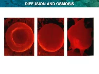
12. Osmotic swelling is an unavoidable problem for all cells • The swelling arises from the presence of negatively-charged proteins trapped in the cytoplasm • First, imagine that a water-permeable membrane separates two rigid compartments. • One compartment has a 150 mmolal concentration of NaCl. • The other one has 150 mEq/liter of Na+ and an equal quantity of anionic charge as protein – however, the protein concentration is only 1 mmolal. • Is there an osmotic gradient? • Is there a solute gradient?

13. Initial conditions Intermediate conditions: Cl- diffused down its gradient; why did Na+ move against its gradient? Notice that there is now a gradient of electrical charge – this is a Donnan potential. Now imagine water trying to move osmotically – is there a gradient of hydrostatic pressure? The system has come into Gibbs-Donnan equilibrium – all forces are balanced.

14. Animal cells could never attain Gibbs-Donnan Equilibrium • Why not? The plasma membrane cannot sustain a hydrostatic pressure gradient. • Without the evolution of some means of avoiding Gibbs-Donnan equilibrium, there would be no protein-containing cells.

15. The Na+/K+ Pump counteracts G-D equilibration The Na+/K+ pump undergoes cycles in which it spends an ATP to eject 3 Na+ from the cell and at the same time to take 2 K+ into the cell. On the average, this counteracts leakage of Na+ and K+ across the membrane down their electrochemical gradients. The bottom-line effect of this is to make the cell effectively impermeable to NaCl. Gibbs-Donnan equilibrium is not approached and the cell does not swell, in spite of the presence of protein anion (X-).

16. What if the Na+/K+ pump stops working?