Download
1 / 45
450 likes | 569 Views
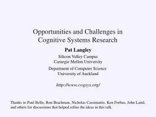
Computational Discovery of Scientific Models: Guiding Search with Knowledge and Data. Pat Langley Department of Computer Science University of Auckland Private Bag 92019 Auckland 1142 NZ.

E N D
Computational Discovery of Scientific Models: Guiding Search with Knowledge and Data Pat Langley Department of Computer Science University of Auckland Private Bag 92019 Auckland 1142 NZ Thanks to K. Arrigo, G. Bradshaw, S. Borrett, W. Bridewell, S. Dzeroski, H. Simon, L. Todorovski, and J. Zytkow for their contributions to this research, which was partly funded by NSF Grant No. IIS-0326059 and ONR Grant No. N00014-11-1-0107.
The Scientific Enterprise Science is a unique collection of activities distinguished by some distinctive characteristics: Systematic collection and analysis of observations Formal statement of theories, laws, andmodels Use of the latter to explain and predict the former Use of observations to evaluate theorized structures Moreover, science can apply these ideas to any area of enquiry, in principle even to science itself.
Philosophy of Science One discipline – philosophy of science – has studied science itself since the 19th Century, including the: character of scientific observations and experiments structure of scientific theories, laws, and models nature of scientific explanations and predictions evaluation of scientific theories, models, and laws However, philosophers of science have typically avoided one important topic: scientific discovery.
Mystical Views of Scientific Discovery Philosophers largely ignored scientific discovery, believing it to be immune to logical analysis. Popper (1934) wrote: The initial stage, the act of conceiving or inventing a theory, seems to me neither to call for logical analysis nor to be susceptible of it … My view may be expressed by saying that every discovery contains an ‘irrational element’, or ‘a creative intuition’… He was not alone in this view. Hempel and many others believed discovery was inherently irrational and beyond understanding. However, advances made by two fields – cognitive psychology and artificial intelligence – in the 1950s suggested otherwise.
Scientific Discovery as Problem Solving Simon (1966) offered another view – that scientific discovery is a variety of problem solving that involves: Search through a space of connected problem states Generated from earlier states by mental operators Guided by heuristics that keep the search tractable Heuristic search had been implicated in many cases of human problem solving, such as proving theorems and playing chess. This idea offered a powerful new approach to understanding the rational character of scientific discovery. But it also suggested ways to automate this mysterious process.
States in the problem space map onto locations in the maze. Operators for producing new states map onto steps through the maze. Solutions correspond to paths from the maze entrance to its exit (goal). Initial state Goal state Heuristic Search in a Problem Space Heuristic search is analogous to the traversal of a physical maze. The initial state and the operators implicitly define a problem space. Heuristics aid search by favoring likely choices and rejecting others to make solution finding tractable.
An Early Response For my CMU dissertation research, I adapted Simon’s ideas on scientific discovery, developing a computer program that: Carried out search in a problem space of theoretical terms; Using operators that combined old terms into new ones; Guided by heuristics that noted regularities in data; and Applied these recursively to formulate higher-level relations. The result was Bacon, an early AI system that rediscovered laws from the history of physics and chemistry. I named the system after Sir Francis Bacon because it adopted a data-driven approach to discovery.
p 1.77 3.57 7.16 16.69 Bacon on Kepler’s Third Law The Bacon system carried out heuristic search, through a space of numeric terms, looking for constants and linear relations. moon d d/p d2/p d3/p2 A 5.67 3.20 18.15 58.15 B 8.67 2.43 21.04 51.06 C 14.00 1.96 27.40 53.61 D 24.67 1.48 36.46 53.89 This table shows its progression from the distance and period of Jupiter’s moons to a term with nearly constant value.
Bacon on the Ideal Gas Law Bacon rediscovered the ideal gas law, PV = aNT + bN, in three stages, each at a different level of description. d = aT + b c/N = d1 c/N = d2 c/N = d3 PV = c1 PV = c2 PV = c3 PV = c4 PV = c5 PV = c6 PV = c7 PV = c8 PV = c9 Parameters for laws at one level became dependent variables in laws at the next level, enabling discovery of complex relations.
Some Laws Discovered by Bacon • Basic algebraic relations: • Ideal gas law PV = aNT + bN • Kepler’s third law D3 = [(A – k) / t]2 = j • Coulomb’s law FD2 / Q1Q2 = c • Ohm’s law TD2 / (LI – rI) = r • Relations with intrinsic properties: • Snell’s law of refraction sin I / sin R = n1 /n2 • Archimedes’ law C = V + i • Momentum conservation m1V1 = m2V2 • Black’s specific heat law c1m1T1 + c2m2T2 = (c1m1+ c2m2 )Tf
Initial Responses to Bacon Responses to the Bacon work were mixed, with some agreeing it clarified important aspects of scientific discovery. But others claimed that thereal key to discovery, which Bacon did not address, instead lay in: Deciding which variables to measure and relate Determining which problem space to search Selecting which scientific problem to address Others held that Bacon only did what it was programmed to do, and thus did not really ‘discover’ anything. We only claimed the system offered insights into the operation of scientific discovery, with much remaining to be done.
Ensuing Systems for Law Discovery Indeed, Bacon inspired other AI systems for law discovery like: • ABACUS (Falkenhainer, 1985) and ARC (Moulet, 1992) • Fahrenheit (Zytkow, Zhu, & Hussam, 1990) • COPER (Kokar, 1986) and E* (Schaffer, 1990) • IDS (Nordhausen & Langley, 1990) • Hume (Gordon & Sleeman, 1992) • DST (Murata, Mizutani, & Shimura, 1994) • SSF (Washio et al., 1997) and LaGramge (Todorovski et al., 2006) • GP (Koza et al., 2001) and Eureqa (Schmidt & Lipson, 2009) These relied on different methods but also searched for explicit mathematical laws that matched data.
1979 1980 1981 1982 1983 1984 1985 1986 1987 1988 1989 1990 1991 1992 1993 1994 1995 1996 1997 1998 1999 2000 Bacon.1–Bacon.5 Abacus, Coper Fahrehneit, E*, Tetrad, IDSN Hume, ARC DST, GPN LaGrange SDS SSF, RF5, LaGramge AM Glauber NGlauber IDSQ, Live RL, Progol HR Dendral Dalton, Stahl Stahlp, Revolver Gell-Mann BR-3, Mendel Pauli BR-4 IE Coast, Phineas, AbE, Kekada Mechem, CDP Astra, GPM Numeric laws Qualitative laws Structural models Process models Other Research on Discovery (from 1979 to 2000) Interest in computational discovery spread to other aspects of science, including qualitative laws and explanatory models. Legend Research in this tradition has continued to the present, in some cases producing new scientific results.
Successes of Computational Scientific Discovery AI systems of this type have helped to discover new knowledge in many scientific fields: • reaction pathways in catalytic chemistry (Valdes-Perez, 1994, 1997) • qualitative chemical factors in mutagenesis (King et al., 1996) • quantitative laws of metallic behavior (Sleeman et al., 1997) • quantitative conjectures in graph theory (Fajtlowicz et al., 1988) • qualitative conjectures in number theory (Colton et al., 2000) • temporal laws of ecological behavior (Todorovski et al., 2000) • models of gene-influenced metabolism in yeast (King et al., 2009) Each of these has led to publications in the refereed literature of the relevant scientific field.
The Data Mining Movement During the 1990s, a new paradigm known as dataminingand knowledge discovery emerged that: Emphasized the availability of large amounts of data; Used computational methods to find regularities in the data; Adopted heuristic search through a space of hypotheses; Initially focused on commercial applications and data sets. Most work used notations invented by computer scientists, unlike work on scientific discovery, which used scientific formalisms. Data mining has been applied to scientific data, but the results seldom bear a resemblance to scientific knowledge.
Discovering Explanatory Models The early stages of any science focus on descriptive laws that summarize empirical regularities. Mature sciences instead emphasize the creation of models that explain phenomena in terms of: • Inferred components and structures of entities • Hypothesized processes about entities’ interactions Explanatory models move beyond description to provide deeper accounts linked to theoretical constructs. Can we develop computational systems that address this more sophisticated side of scientific discovery?
An Example: The Ross Sea Ecosystem Formal accounts of ecosystem dynamics are often cast as sets of differential equations. Here four equations describe the concentrations of phytoplankton, zooplankton, nitrogen, and detritus in the Ross Sea over time. Such models can match observed variables with some accuracy. d[phyto,t,1] = 0.307 phyto 0.495 zoo + 0.411 phyto d[zoo,t,1] = 0.251 zoo + 0.615 0.495 zoo d[detritus,t,1] = 0.307 phyto +0.251 zoo + 0.385 0.495 zoo 0.005 detritus d[nitro,t,1] = 0.098 0.411 phyto + 0.005 detritus
A Deeper Account of Ross Sea Dynamics As phytoplankton uptakes nitrogen, its concentration increases and the nitrogen decreases. This continues until the nitrogen is exhausted, which leads to a phytoplankton die off. This produces detritus, which gradually remineralizes to replenish nitrogen. Zooplankton grazes on phytoplankton, which slows the latter’s increase and also produces detritus. d[phyto,t,1] = 0.307 phyto 0.495 zoo + 0.411 phyto d[zoo,t,1] = 0.251 zoo + 0.615 0.495 zoo d[detritus,t,1] = 0.307 phyto +0.251 zoo + 0.385 0.495 zoo 0.005 detritus d[nitro,t,1] = 0.098 0.411 phyto + 0.005 detritus
Processes in Ross Sea Dynamics As phytoplankton uptakes nitrogen, its concentration increases and the nitrogen decreases. This continues until the nitrogen is exhausted, which leads to a phytoplankton die off. This produces detritus, which gradually remineralizes to replenish nitrogen. Zooplankton grazes on phytoplankton, which slows the latter’s increase and also produces detritus. d[phyto,t,1] = 0.307 phyto 0.495 zoo + 0.411 phyto d[zoo,t,1] = 0.251 zoo + 0.615 0.495 zoo d[detritus,t,1] = 0.307 phyto +0.251 zoo + 0.385 0.495 zoo 0.005 detritus d[nitro,t,1] = – 0.098 0.411 phyto + 0.005 detritus
Processes in Ross Sea Dynamics As phytoplankton uptakes nitrogen, its concentration increases and the nitrogen decreases. This continues until the nitrogen is exhausted, which leads to a phytoplankton die off. This produces detritus, which gradually remineralizes to replenish nitrogen. Zooplankton grazes on phytoplankton, which slows the latter’s increase and also produces detritus. d[phyto,t,1] = 0.307 phyto 0.495 zoo + 0.411 phyto d[zoo,t,1] = 0.251 zoo + 0.615 0.495 zoo d[detritus,t,1] = 0.307 phyto +0.251 zoo + 0.385 0.495 zoo 0.005 detritus d[nitro,t,1] = 0.098 0.411 phyto + 0.005 detritus
model Ross_Sea_Ecosystem entities: phyto, zoo, nitro, detritus observables: phyto, nitro process phyto_loss(phyto, detritus) equations: d[phyto.conc,t,1] = 0.307 phyto.conc d[detritus.conc,t,1] = 0.307 phyto.conc process zoo_loss(zoo, detritus) equations: d[zoo.conc,t,1] = 0.251 zoo.conc d[detritus.conc,t,1] = 0.251 zoo.conc process zoo_phyto_grazing(zoo, phyto, detritus) equations: d[zoo.conc,t,1] = 0.615 0.495 zoo.conc d[detritus.conc,t,1] = 0.385 0.495 zoo.conc d[phyto.conc,t,1] = 0.495 zoo.conc process nitro_uptake(phyto, nitro) equations: d[phyto.conc,t,1] = 0.411 phyto.conc d[nitro.conc,t,1] = 0.098 0.411 phyto.conc process nitro_remineralization(nitro, detritus) equations: d[nitro.conc,t,1] = 0.005 detritus.conc d[detritus.conc,t,1 ] = 0.005 detritus.conc A Process Model for the Ross Sea We can reformulate such an account by restating it as a quantitative process model. Such a model is equivalent to a standard differential equation model, but it makes explicit assumptions about processes that are involved. Each process indicates that certain terms in equations must stand or fall together.
A New Discovery Task We can define the task of discovering such explanatory process models as: Given: A set of entities with associated variables Given: Times series for some of these variables Given: Knowledge about processes that might occur Find: Quantitative process models that explain the observed time series and predict new observations We have referred to this class of computational discovery tasks as inductive process modeling(Bridewell et al., 2008).
model AquaticEcosystem variables: nitro, phyto, zoo, nutrient_nitro, nutrient_phyto observables: nitro, phyto, zoo process phyto_exponential_growth equations: d[phyto,t] = 0.1 phyto process zoo_logistic_growth equations: d[zoo,t] = 0.1 zoo / (1 zoo / 1.5) process phyto_nitro_consumption equations: d[nitro,t] = 1 phyto nutrient_nitro, d[phyto,t] = 1 phyto nutrient_nitro process phyto_nitro_no_saturation equations: nutrient_nitro = nitro process zoo_phyto_consumption equations: d[phyto,t] = 1 zoo nutrient_phyto, d[zoo,t] = 1 zoo nutrient_phyto process zoo_phyto_saturation equations: nutrient_phyto = phyto / (phyto + 0.5) process exponential_growth variables: P {population} equations: d[P,t] = [0, 1,] P process logistic_growth variables: P {population} equations: d[P,t] = [0, 1, ] P (1 P / [0, 1, ]) process constant_inflow variables: I {inorganic_nutrient} equations: d[I,t] = [0, 1, ] process consumption variables: P1 {population}, P2 {population}, nutrient_P2 equations: d[P1,t] = [0, 1, ] P1 nutrient_P2, d[P2,t] = [0, 1, ] P1 nutrient_P2 process no_saturation variables: P {number}, nutrient_P {number} equations: nutrient_P = P process saturation variables: P {number}, nutrient_P {number} equations: nutrient_P = P / (P + [0, 1, ]) observations Inductive Process Modeling process model Heuristic Search phyto, nitro, zoo, nutrient_nitro, nutrient_phyto generic processes entities
process exponential_loss(S, D) process remineralization(N, D) entities: S{species}, D{detritus} entities: N{nutrient}, D{detritus} parameters: [0, 1] parameters: [0, 1] equations: d[S.conc,t,1] = 1 S.conc equations: d[D.conc,t,1] = S.conc d[N.conc, t,1] = D.conc d[D.conc, t,1] = 1 D.conc generic process grazing(S1, S2, D) process constant_inflow(N) entities: S1{species}, S2{species}, D{detritus} entities: N{nutrient} parameters: [0, 1], [0, 1] parameters: [0, 1] equations: d[S1.conc,t,1] = S1.conc equations: d[N.conc,t,1] = d[D.conc,t,1] = (1 ) S1.conc d[S2.conc,t,1] = 1 S1.conc generic process nutrient_uptake(S, N) entities: S{species}, N{nutrient} parameters: [0, ], [0, 1], [0, 1] conditions: N.conc > equations: d[S.conc,t,1] = S.conc d[N.conc,t,1] = 1 S.conc Generic Processes for Aquatic Ecosystems Our aquatic ecosystem library contains about 25 generic processes, including ones with alternative functional forms for loss and grazing processes. These form the building blocks from which to compose models.
We have developed multiple ‘IPM’ systems that induce process models from generic components in four stages: Searching the Space of Model Structures 1. Instantiate known generic processes with specific entities, subject to type specifications; 2. Combine these instantiated processes into candidate model structures, rejecting disconnected structures; 3. For each model structure, carry out search through parameter space to find good coefficients; 4. Return the parameterized model with the best overall score (e.g., lowest squared error). We have reported variants on this approach in numerous papers (Bridewell et al., MLj, 2008; Bridewell & Langley, TopiCS, 2010).
To estimate the parameters for each generic model structure, our induction algorithms: Searching the Space of Model Parameters 1. Select random initial values that fall within ranges specified in the generic processes; 2. Improve these parameters using a conjugate gradient method (717) until it reaches a local optimum; 3. Repeat the process ten times and select the best-scoring set of parameter values. This multi-level method gives reasonable fits to time-series data from a number of domains, but it is computationally intensive. Each step in the gradient descent requires simulating the model’s trajectory to calculate its error.
Results on Training Data from Ross Sea We provided IPM with 188 samples of phytoplankton, nitrate, and ice measures taken from the Ross Sea. From 2035 distinct model structures, it found accurate models that limited phyto growth by the nitrate and the light available. Some high-ranking models incorporated zooplankton, whereas others did not.
Results on Test Data from Ross Sea Generalization to a second year’s data benefited from treating initial zooplankton concentration as a free model parameter. Another good-fitting model suggested that the nitrogen to carbon ratio varies as a function of available light.
Other Results with Process Modeling protist dynamics power systems biochemical kinetics hydrology
In addition, we have extended the basic framework to support: Extensions to Inductive Process Modeling Inductive revision of quantitative process models Asgharbeygi et al. (Ecological Modeling, 2006) Hierarchical generic processes that constrain search Todorovski, Bridewell, Shiran, and Langley (AAAI-2005) An ensemble-like method that mitigates overfitting effects Bridewell, Bani Asadi, Langley, and Todorovski (ICML-2005) An EM-like method that estimates missing observations Bridewell, Langley, Racunas, and Borrett (ECML-2006) These extensions make the modeling framework more robust along a number of fronts.
Because few scientists want to be replaced, we also developed an interactive environment, PROMETHEUS, that lets users: Interfacing with Scientists specify a quantitative process model of the target system; display and edit the model’s structure and details graphically; simulate the model’s behavior over time and situations; compare the model’s predicted behavior to observations; invoke a revision module in response to detected anomalies. The environment offers computational assistance in forming and evaluating models but lets the user retain control.
The PROMETHEUS System Details about PROMETHEUSare available in Bridewell et al.(IJHCS, 2007).
Knowledge and Search in Discovery • Traditional treatments of problem solving hold that knowledge reduces the amount of search. • But adding generic processes leads to a combinatorial increase in the number of candidate structures. • Yet scientists are not overwhelmed by the size of model spaces and they reject many structures as unacceptable. This suggests two forms of scientific background knowledge: • components used to generate candidate model structures • constraints on allowable combinations of such components • This distinction seldom occurs in the literature, but it appears key to understanding scientific explanation.
Constraints on Ecosystem Models Our discussions with ecologists confirmed that constraints play an important role in model acceptability. Some plausible constraints for models of ecosystems include: We have developed a formal notation that lets our systems use such constraints during inductive process modeling. • There must be at most one growth process for each species. • A limited growth process cannot occur without a nutrient limitation process and vice versa. • There must be no more than one predation process between any two species.
model AquaticEcosystem variables: nitro, phyto, zoo, nutrient_nitro, nutrient_phyto observables: nitro, phyto, zoo process phyto_exponential_growth equations: d[phyto,t] = 0.1 phyto process zoo_logistic_growth equations: d[zoo,t] = 0.1 zoo / (1 zoo / 1.5) process phyto_nitro_consumption equations: d[nitro,t] = 1 phyto nutrient_nitro, d[phyto,t] = 1 phyto nutrient_nitro process phyto_nitro_no_saturation equations: nutrient_nitro = nitro process zoo_phyto_consumption equations: d[phyto,t] = 1 zoo nutrient_phyto, d[zoo,t] = 1 zoo nutrient_phyto process zoo_phyto_saturation equations: nutrient_phyto = phyto / (phyto + 0.5) process exponential_growth variables: P {population} equations: d[P,t] = [0, 1,] P process logistic_growth variables: P {population} equations: d[P,t] = [0, 1, ] P (1 P / [0, 1, ]) process constant_inflow variables: I {inorganic_nutrient} equations: d[I,t] = [0, 1, ] process consumption variables: P1 {population}, P2 {population}, nutrient_P2 equations: d[P1,t] = [0, 1, ] P1 nutrient_P2, d[P2,t] = [0, 1, ] P1 nutrient_P2 process no_saturation variables: P {number}, nutrient_P {number} equations: nutrient_P = P process saturation variables: P {number}, nutrient_P {number} equations: nutrient_P = P / (P + [0, 1, ]) observations Reduction in search space entities Inductive Process Modeling phyto, nitro, zoo, nutrient_nitro, nutrient_phyto process model Heuristic Search Heuristic Search constraints Always-together[growth(P), loss(P)] Exactly-one[lotka-volterra(P, G), ivlev(P, G), watts(P, G)] At-most-one[photoinhibition(P, E)] Necessary[nutrient-mixing(N), remineralization(N, D)] generic processes
Our extended framework for the discovery of process models: Inducing Process Models with Constraints Encodes modular constraints on process combinations Uses these constraints to eliminate unacceptable models Reduces search through the model space, which Leads to far more efficient model construction Produces little or no increase in generalization error Improves the comprehensibility of generated models The resulting systems are more robust in their ability to induce process models (Bridewell & Langley, TopiCS, 2010).
In other recent work (Todorovski et al., AAAI-2012), we have developed a system that: Discovering Constraints Uses inductive process modeling to generate a set of models; Separates these into accurate and inaccurate model structures; Describes each model structure in terms of relational literals; Learns relational rules that can distinguish the two classes; Transforms the rules into constraints on model structures; and Uses these constraints to guide search on future modeling tasks. Experiments suggests this produces a tenfold speedup on novel modeling tasks with little or no loss in accuracy.
Despite the progress to date, we need further work in order to: Directions for Future Research apply approach to new data sets (oceanography, physiology) develop more efficient methods for fitting model parameters extend the framework to partial differential equation models design mechanisms for inducing new generic processes handle discovery of complex models with many variables embed these abilities in a PROMETHEUS-like environment Together, these will make constraint-guided inductive process modeling a more robust approach to scientific explanation.
Inductive process modeling is a novel and promising approach to discovering scientific models that: Summary Remarks Incorporates a formalism that is familiar to many scientists Utilizes two kinds of background knowledge about the domain Produces meaningful results from moderate amounts of data Generates models that explain, not just describe, observations Closes the loop between using and learning process constraints Although work on this topic has focused on ecological modeling, the key ideas extend to other domains. For more information, see http://www.isle.org/process/ .
eScience and Discovery Informatics The escience movement champions the use of computers to aid the scientific enterprise, emphasizing two themes: • Collection, storage, and mining of scientific data sets • E.g., learned classifiers in astronomy and planetology • But such analyses make no contact with scientific theory Creation and simulation of complex explanatory models E.g., differential equation models formeteorology and biology However, most such models are constructed manually Science is about the relation between theory and data, and work on computational scientific discovery offers a way to join them. This idea is central to the emerging field of discovery informatics.
Digital collection and storage have led to rapid growth of data in many areas. The big data movement seeks to capitalize on this content, but, in science at least, must address three distinct issues: Big Data and Scientific Discovery Scaling to large and heterogeneous data sets Scaling to large and complex scientific models Scaling to large spacesof candidate models Handling large data sets has been widely studied and poses the fewest challenges. We need more work on the last two issues, for which the methods of computational scientific discovery are well suited.
Concluding Remarks Scientific discovery does not involve any mystical or irrational elements; we can study and even partially automate it. Our explanation of this fascinating set of processes relies on: • Carrying out search through a space of laws or models; • Utilizing operators for generating structures and parameters; • Guiding search by data and by knowledge about the domain. Work in this framework discovers laws and models stated in the formalisms and concepts familiar to scientists. This paradigm has already started to aid the scientific enterprise, and its importance will only grow with time.
Publications on Computational Scientific Discovery Bridewell, W., & Langley, P. (2010). Two kinds of knowledge in scientific discovery. Topics in Cognitive Science, 2, 36–52. Bridewell, W., Langley, P., Todorovski, L., & Dzeroski, S. (2008). Inductive process modeling. Machine Learning, 71, 1-32. Bridewell, W., Sanchez, J. N., Langley, P., & Billman, D. (2006). An interactive environment for the modeling and discovery of scientific knowledge. International Journal of Human-Computer Studies, 64, 1099-1114. Dzeroski, S., Langley, P., & Todorovski, L. (2007). Computational discovery of scientific knowledge. In S. Dzeroski & L. Todorovski (Eds.), Computational discovery of communicable scientific knowledge. Berlin: Springer. Langley, P. (2000). The computational support of scientific discovery. International Journal of Human-Computer Studies, 53, 393–410. Langley, P., Simon, H. A., Bradshaw, G. L., & Zytkow, J. M. (1987). Scientific discovery: Computational explorations of the creative processes. Cambridge, MA: MIT Press. Langley, P., & Zytkow, J. M. (1989). Data-driven approaches to empirical discovery. Arti-ficial Intelligence, 40, 283–312. Todorovski, L., Bridewell, W., & Langley, P. (2012). Discovering constraints for inductive process modeling. Proceedings of the Twenty-Sixth AAAI Conference on Artificial Intelligence. Toronto: AAAI Press.
In Memoriam In 2001, the field of computational scientific discovery lost two of its founding fathers. Herbert A. Simon (1916 – 2001) Jan M. Zytkow (1945 – 2001) Both were interdisciplinary researchers who published in computer science, psychology, philosophy, and statistics. Herb Simon and Jan Zytkow were excellent role models for us all.