Download
1 / 43
460 likes | 674 Views
(2) Parallel streamlines. (3.1). CHAPTER 3. EXACT ONE-DIMENSIONAL SOLUTIONS. 3.1 Introduction. · Temperature solution depends on velocity · Velocity is governed by non-linear Navier-Stokes eqs. · Exact solution are based on simplifications governing equations .

E N D
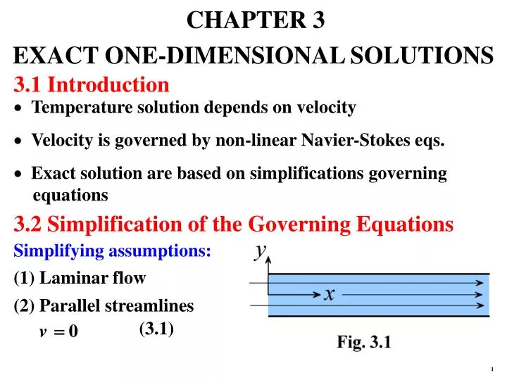
(2) Parallel streamlines (3.1) CHAPTER 3 EXACT ONE-DIMENSIONAL SOLUTIONS 3.1 Introduction ·Temperature solution depends on velocity ·Velocity is governed by non-linear Navier-Stokes eqs. ·Exact solution are based on simplifications governing equations 3.2 Simplification of the Governing Equations Simplifying assumptions: (1) Laminar flow 1
, everywhere (3.2) (3.3) (3.4) (3.5) , everywhere (3.1) into continuity for 2-D, constant density fluid: (3) Negligible axial variation of temperature (3.4) is valid under certain conditions. It follows that (4) Constant properties: velocity and temperature fields are uncoupled (Table 2.1, white box) 2
3.3 Exact Solutions (3.6) (3.7) Fig. 3.2: ·Shaft rotates inside sleeve ·Streamlines are concentric circles ·Axisymmetric conditions, no axial variations 3.3.1 Couette Flow ·Flow between parallel plate ·Motion due to pressure drop and/or moving plate ·Channel is infinitely long 4
Example 3.1: Couette Flow with Dissipation ·Very large parallel plates ·Incompressible fluid ·Upper plate at To moves with velocity Uo ·Insulate lower plate ·Account for dissipation ·Laminar flow, no gravity, no pressure drop ·Determine temperature distribution (1) Observations ·Plate sets fluid in motion ·No axial variation of flow ·Incompressible fluid ·Cartesian geometry 5
(2) Problem Definition. Determine the velocity and temperature distribution (3) Solution Plan ·Find flow field, apply continuity and Navier-Stokes equations ·Apply the energy to determine the temperature distribution (4) Plan Execution (i) Assumptions ·Steady state ·Laminar flow ·Constant properties ·Infinite plates ·No end effects ·Uniform pressure ·No gravity 6
(ii) Analysis (3.19b) is dissipation (3.17) Start with the energy equation 7
(2.2b) (a) (b) (c) (d) Need u, v and w. Apply continuity and the Navier-Stokes equations Continuity Constant density Infinite plates (a) and (b) into (2.2b) Integrate (c) 8
(e) (f) is “constant” of integration Streamlines are parallel (2.10x) Apply the no-slip condition (d) and (e) give Substitute into (d) To determine u we apply the Navier-Stokes eqs. 9
(g) (h) (i) (j) (k) and (l) Simplify: Steady state No gravity Negligible axial pressure variation (b) and (f)-(i) into (2.10x) gives Solution to (j) is Boundary conditions 10
(m) (3.8) and (n) (o) Steady state: (k) and (I) give (m) into (k) Dissipation: (b) and (f) into (2.17) Use (3.8) into (n) Infinite plates at uniform temperature: 11
(p) (q) (r) and (s) and (3.9) Use above, (b), (f) and (o) into energy (2.10b) Integrate B.C. B.C. and solution (q) give (s) into (q) 12
(3.10) Fourier’s law gives heat flux at y = H (3.9) into the above (iii) Checking Dimensional check: Each term in (3.8) and (3.9) is dimensionless. Units of (3.10) is W/m2 Differential equation check: Velocity solution (3.8) satisfies (j) and temperature solution (3.9) satisfies (p) Boundary conditions check: Solution (3.8) satisfies B.C. (l), temperature solution (3.9) satisfies B.C. (r) 13
(ii) Stationary upper plate: no dissipation, uniform temperature To, no surface flux. Set Uo = 0 in (o), (3.9) and (3.10) gives T(y) = To and (iii) Inviscid fluid: no dissipation, uniform temperature To. Set in (3.9) gives T(y) = To = Friction work by plate = Heat conducted through plate (t) Limiting check: (i) Stationary upper plate: no fluid motion. Set Uo = 0 in (3.8) gives u(y) = 0 (iv) Global conservation of energy: Frictional energy is conducted through moving plate: where 14
(u) (v) (w) = shearing stress (3.8) into (u) (v) and (t) (w) agrees with (3.10) (4) Comments ·Infinite plate is key assumption. This eliminates x as a variable ·Maximum temperature: at y = 0 Set y = 0 in (3.9) 15
3.3.2 Hagen-Poiseuille Flow ·Motion is due to pressure gradient ·Problems associated with axial flow in channels ·Motion due to pressure drop ·Channel is infinitely long Example 3.2: Flow in a Tube at Uniform Surface Temperature ·Incompressible fluid flows in a long tube ·Surface temperature To ·Account for dissipation ·Assuming axisymmetric laminar flow 16
[c] Nusselt number based on [ ] ·Neglecting gravity and end effects ·Determine: [a] Temperature distribution [b] Surface heat flux (1) Observations ·Motion is due to pressure drop ·Long tube: No axial variation ·Incompressible fluid ·Heat generation due to dissipation ·Dissipated energy is removed by conduction at the surface ·Heat flux and heat transfer coefficient depend on temperature distribution 17
·Temperature distribution depends on the velocity distribution ·Cylindrical geometry (2) Problem Definition. Determine the velocity and temperature distribution. (3)Solution Plan ·Apply continuity and Navier-Stokes to determine flow field ·Apply energy equation to determine temperature distribution ·Fourier’s law surface heat flux ·Equation (1.10) gives the heat transfer coefficient. (4) Plan Execution 18
(i) Assumptions (2.24) ·Steady state ·Laminar flow ·Axisymmetric flow ·Constant properties ·No end effects ·Uniform surface temperature ·Negligible gravitational effect (ii) Analysis [a] Start with energy equation (2.24) 19
(2.25) ·Need , and (2.4) Constant (a) (b) where ·Flow field: use continuity and Navier-Stokes eqs. Axisymmetric flow 20
(c) (d) (e) is “constant” of integration. Use the no-slip B.C. (f) (g) Streamlines are parallel Determine : Navier-Stokes eq. in z-direction Long tube, no end effects (a)-(c) into (2.4) Integrate (e) and (f) give Substitute into (e) 21
(2.11z) (h) (i) (3.11) depends on r only, rewrite (3.11) (j) Simplify Steady state: No gravity: (b), (c) and (g)-(i) into (2.11z) 22
(k) (2.11r) (l) (m) = “constant” of integration Integrate Apply Navier-Stokes in r-direction (b), (g) and (i) into (2.11r) Integrate ·Equate two solutions for p: (k) and (m): 23
(n) g(r) = C (o) (p) (q) Two B.C. on : (r) C = constant. Use (o) into (j) Integrate integrate again (q) and (r) give C1and C2 24
(3.12) (s) (t) Substitute into (q) For long tube at uniform temperature: (b), (c), (g), (h) and (s) into energy (2.24) (b), (c) and (g) into (2.25) Substitute velocity solution (3.11) into the above 25
(u) (3.13) (v) (w) (3.14a) (u) in (t) and rearrange Integrate Need two B.C. (v) and (w) give Substitute into (v) 26
(3.14b) (3.15) (x) (y) In dimensionless form: [b] Use Fourier’s (3.14) into above [c] Nusselt number: (1.10) gives h (3.14a) into (y) 27
(z) (3.16) (z) into (x) (iii) Checking Dimensional check: ·Each term in (3.12) has units of velocity ·Each term in (3.14a) has units of temperature ·Each term in (3.15) has units of W/m2 Differential equation check: Velocity solution (3.12) satisfies (p) and temperature solution (3.14) satisfies (3.13) Boundary conditions check: Velocity solution (3.12) satisfies B.C. (r) and temperature solution (3.14) satisfies B.C. (w) Limiting check: 28
(ii) Uniform pressure ( ): No fluid motion, no dissipation, no surface flux. Set in (3.15) gives (i) Uniform pressure ( ): No fluid motion. Set in (3.12) gives (z-1) = upstream pressure = downstream pressure = flow rate (iii) Global conservation of energy: Pump workW for a tube of lengthL 29
(z-2) (z-3) Work per unit area (z-4) (3.12) into the above, integrate (z-1) and (z-2) (z-3) into the above However Combine with (z-4) 30
This agrees with (3.15) (5) Comments ·Key simplification: long tube with end effects. This is same as assuming parallel streamlines ·According to (3.14), maximum temperature is at center r = 0 ·The Nusselt number is constant independent of Reynolds and Prandtl numbers 31
Example 3.3: Lubrication Oil Temperature in RotatingShaft ·Angular velocity is 3.3.3 Rotating Flow ·Lubrication oil between shaft and housing ·Assuming laminar flow ·Account for dissipation ·Determine the maximum temperature rise in oil (1) Observations ·Fluid motion is due to shaft rotation ·Housing is stationary 32
·Constant ·No axial variation in velocity and temperature ·No variation with angular position ·Frictional heat is removed at housing ·No heat is conducted through shaft ·Maximum temperature at shaft ·Cylindrical geometry (2) Problem Definition. Determine the velocity and temperature distribution of oil (3) Solution Plan ·Apply continuity and Navier-Stokes eqs. to determine flow field ·Use energy equation to determine temperature field ·Fourier’s law at the housing gives frictional heat 33
(2.24) (4) Plan Execution (i) Assumptions ·Steady state ·Laminar flow ·Axisymmetric flow ·Constant properties ·No end effects ·Uniform surface temperature ·Negligible gravitational effect (ii) Analysis ·Energy equation governs temperature 34
where (2.25) Need flow field , and (2.4) Constant (a) (b) ·Apply continuity and Navier-Stokes to determine flow field Axisymmetric flow 35
(c) (d) (e) (f) (g) Apply the Navier-Stokes to determine Streamlines are concentric circles Long shaft: (a)-(c) into (2.4) Integrate Apply B.C. to determine C (e) and (f) give C = 0 Use (e) 36
(2.11 ) (h) Neglect gravity, use (b),(c), (g), (h) into (2.11 ) (3.17) (i) (j) For steady state: Integrate B.C. are 37
(k) (3.18) (j) gives and (l) (k) into (i) Simplify energy equation (2.24) and dissipation function (2.25). Use(b), (c), (g), (h) and (3.18) into above 38
(m) (3.19) (n) (o) and (n) and (o) give and Combine (m) and (l) Integrate(3.19) twice Need two B.C. 39
(3.20a) (3.20b) Maximum temperature at (3.21) Use Fourier’s law to determine frictional energy per unit length Substitute into (o) or 40
(3.22) (3.20a) in above (iii) Checking ·Each term in solutions (3.18) and (3.20b) is dimensionless ·Equation (p) has the correct units of W/m Differential equation check: ·Velocity solution (3.18) satisfies (3.17) and temperature solution (3.20) satisfies (3.19) Boundary conditions check: ·Velocity solution (3.18) satisfies B.C. (j) and temperature solution (3.20) satisfies B.C. (o) 41
·Stationary shaft: No fluid motion. Set in (3.18) gives (p) = shearing stress ·Stationary shaft: No dissipation, no heat loss Set in (3.22) gives (q) (r) Limiting check: ·Global conservation of energy: Shaft work per unit length (3.18) into the above 42
(s) ·Single governing parameter: Combining (p) and (r) This is identical to surface heat transfer (3.22) (5) Comments ·The key simplifying assumption is axisymmetry ·Temperature rise due to frictional heat increase as the clearance s decreased 43