Download
1 / 60
600 likes | 823 Views
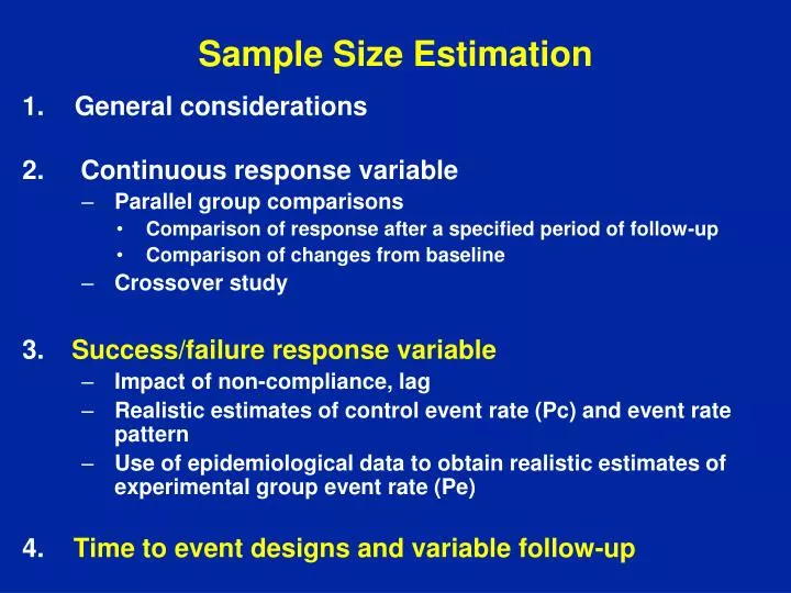
Sample Size Estimation. 1. General considerations 2. Continuous response variable Parallel group comparisons Comparison of response after a specified period of follow-up Comparison of changes from baseline Crossover study 3. Success/failure response variable

E N D
Sample Size Estimation 1.General considerations 2. Continuous response variable • Parallel group comparisons • Comparison of response after a specified period of follow-up • Comparison of changes from baseline • Crossover study 3. Success/failure response variable • Impact of non-compliance, lag • Realistic estimates of control event rate (Pc) and event rate pattern • Use of epidemiological data to obtain realistic estimates of experimental group event rate (Pe) 4. Time to event designs and variable follow-up
( ) 2 2 s 2 z + z a b 1 - /2 1 - n = 2 D Comparison of Sample Size Formulae for Means and Proportions (n per group) For means:
Example • H0: Pc= Pe (proportion with event on control arm = proportion with event on experimental arm) • HA: Pc= .40, Pe = .30 = .40 - .30 = .10 • Assume a = .05 Za = 1.96 (2-sided) 1 - b = .90 Zb = 1.28 • p = (.40 + .30 )/2 = .35
Example (cont.) N = 476; 2N = 952
Approximate* Total Sample Size for Comparing Proportions in Two Groups of Equal Size with Significance Level () of 0.05 and Power (1- ) of 0.90 PC (Control Group) PE (Experimental Group) Total Sample Size 0.50 0.40 1040 0.30 250 0.20 110 0.30 0.20 790 0.15 330 0.10 170 0.10 0.08 8600 0.05 1170 0.02 370 0.05 0.03 4030 0.025 2430 0.01 760 0.03 0.015 4100 0.03 0.019 8290 0.03 0.02 10240 0.019 0.013 18360 Similar to MRFIT * Sample sizes are rounded up to the nearest 10.
Factors Which Influence “Realized Delta Pc-Pe”(Delta = Hypothesized Treatment Difference) • Non-compliance to experimental treatment • Switchover from control to experimental treatment • Lag time for experimental treatment to influence endpoint • Events counted as an endpoint that are not influenced by treatments under study (e.g., accidental or violent deaths in a study of HIV treatments)
Strategy for Specifying Delta and Estimating Sample Size • Begin by specifying the minimal effect of experimental treatment which would be considered clinically relevant (usually this is done in terms of a relative difference, e.g., relative risk or hazard ratio) • Assume immediate full impact of treatment on endpoint and full compliance • Adjust this “optimistic delta” downwards for non-compliance and lag if necessary • Calculate sample size using “adjusted delta” • Inflate sample size (again) for competing events and losses • For planned sample size, assess impact of deviations from “adjusted delta” on power
No. competing events Losses No. primary events Standardization 2 x Variability x [Constant (,)]2 Delta2 N Per Group = Clinical judgement Lag Biologic plausibility Non-compliance
Simple Adjustment for Non-Compliance in Experimental Group Example: Heart failure trial; primary endpoint is death or hospitalization for heart failure. PC = 0.30 (Placebo group event rate) after 3 years Pe = 0.24 (New treatment event rate) after 3 years • Assume 20% of patients do not comply with experimental treatment (d) • Assume risk of endpoint for non-compliers in experimental group is the same as placebo group
P P P c e e P e ∆ NEW ∆ OLD Simple Adjustment for Non-Compliance = 0.20 ( ) + 0.80 ( ) ADJ = 0.252 ADJ = 0.30 - 0.252 = 0.048; = 0.30 - 0.24 = 0.06 Unadjusted sample size = 1150 per group Approximation: Inflate usual sample size by 1 2 (1-d) where d = fraction of patients not complying 1 ( ) 2 New sample size = 1150 ≈ 1800 per group (.8)
Compliance Adjustment d = fraction who do not comply to exp. treatment P dP ( 1 d)P e c e ADJ P P ( 1 d)(P P ) c e c e ADJ Inflate usual sample size by 1 2 (1 - d)
TOXO Study DesignPower to Detect a 50% Differencefor Sample Size of 265 Patients 0 0 0.80 10 0.74 25 0.66 10 0 0.75 10 0.71 25 0.63 25 0 0.69 10 0.65 25 0.57 Switchover from placebo to active Non-compliance to Pyrimethamine Power
Realistic Estimates of Pe and Pc • Halperin M, J Chronic Dis,1968 (constant event rates for control and experimental groups, non-compliance in experimental group and lag) • Wu M, Cont Clin Trials,1980 (extended Halperin’s method to non-compliance in control group and time-dependent non-compliance) • Lakatos E, Cont Clin Trials,1986 and Biometrics, 1988 (extended to log rank test – time to event analyses) • Shih J, Cont Clin Trials,1995 and Encyclopedia of Clinical Trials, 2007 (implemented Lakatos methods in SAS – Size program – allows event rates to vary and extended to weighted log rank and unequal allocation)
Definitions Dropout – Non-compliance to exp. treatment Dropin – Non-compliance to control treatment Lag – Time for treatment to achieve maximum benefit Lost-to-follow-up – A person for whom endpoint status is unknown (outcome is missing)
P c P e P e Halperin Model to Adjust for Non-Compliance and Lag in Experimental Group 1. Specify 2. Specify (or k); k = where k x 100 = % reduction in control group event rate due to experimental treatment 3. Specify nonadherence rate in experimental group: d 4. Specify lag: f 5. Obtain adjusted value of from table 6. Obtain inflated sample size estimate Pc - PePc
d x Cumulative Dropout Rate T 0 Later development: allow pattern of dropout to vary over follow-up of length T x d Cumulative Dropout Rate 0 T
Effect of Non-adherence on Pe c c = hazard for controls e = hazard for experimental group Non-Dropouts e 0 T Dropouts assume the risk of participants in the control arm. Their risk reverts in the same manner as it decreased before dropout (immediately if lag=0)
Lag -- Halperin defined r (t), the hazard of event in experimental group, as follows: kt f c(1- ), t < f { r(t) = c(1- k) = e, t > f Linear decline to e between T=0 and T=f c e 0 f T Halperin M, et al give tables for f=0, 0.5T, T and 2T.
Example: Heart Failure Trial with Death or Hospitalization for Heart Failure as Primary Endpoint p = 0.30 K = 0.20 c Assume event rate is 30% after 3 years; event rate is constant; 20% of those assigned new treatment will discontinue it after 3 years (cumulative dropout=20%; and there is no lag. p = 0.24 e d = 0.20 = 0) Table 1 of Halperin (f p = 0.246 K 0.18 = Adj. e N = 1425 per group Before we had p = 0.252 e ADJ N = 1800 per group
p = 0.30 c p = 0.24 e k = 0.20 d = 0.20 = 0 f Impact of Dropout Pattern on pe and k:Heart Failure Example (cont.) (1,1,1,1,1,1,1,1) (Halperin) 0.246 0.180 (2,1,1,1,1,1,1,1) 0.247 0.177 (1,0,0,0,0,0,0,0) 0.251 0.163 (1,1,1,1,1,1,1,2) 0.246 0.181 (0,0,0,0,0,0,0,1) 0.241 0.197 Pattern of Dropout Over Four Years (Eight 6-Month Time Periods Adjusted pe Adjusted k
Comparison of Non-AdherenceAdjustments on Sample Size for Heart Failure Trial No adjustment .240 1150 Simple adjustment .252 1800 (instantaneous non-compliance) Halperin (equal over .246 1425 follow-up) Wu/Shih (twice as .247 1485 much in 1st year) Adj. pe N Per Group
Dropout Assumptionsin Major Trials 1. MRFIT (J Chronic Dis, 1977): 50% (2,1,1,1,1,1) 2. CPPT (JAMA, 1984): 35% (1,1,1,1,1,1,1) • Systolic Hypertension in the Elderly (SHEP) (J ClinEpid, 1988): 16% (2,1,1,1,1)
0.50 K 0 0 T/2 T p c p e p e (f = 3) = 8290 versus 4100 with no lag adjustment; alpha=0.05 (2-sided) and power=0.90. 2N NEW Example: Similar to MRFIT (Lag of 3 years)Full Effect of Treatment is 50% and is Reached in 1/2 T = 0.03 (CHD death) K = 0.50 = 0.015 = 0.05, 1- = 0.90 d = 0 (no dropouts) = 6 years, f = 3 years T Adjusted = 0.019 instead of 0.015
Adjustment for Both Non-Compliance and Lag (Parameters Similar to MRFIT) p = 0.03; K = 0.50; = 0.05 (2-sided), 1- = 0.90 T = 6 years; f = 3 years (0.5T); d = 0.50 Adjusted pe = 0.022 2N = 16,610 and 2N = 4100 (no adjustment for lag or dropout) c OLD NEW J Chron Dis 1976. Actually, MRFIT was designed as 1-sided test with alpha=0.05 with unadjusted K=0.542.
Dropout and Dropin Assumptionsin Major Cardiovascular Trials 1. MRFIT 50 0 2. CPPT 35 0 3. SHEP 16 19 Dropout (%) Dropin (%)
Impact of Dropout, Dropin and LagAssumptions on Hypothesized Risk Reductions MRFIT 54% 27% CPPT – 36% SHEP 40% 32% Unadjusted Adjusted
ExampleTOXO Protocol 1. Primary endpoint: Toxoplasmic encephalitis (TE) 2. Control (placebo) group event rate: 30% in 2.5 years 3. Experimental (pyrimethamine) group event rate: 15% in 2.5 years (50% reduction) 4. Death rate unrelated to TE: 33% 5. Confidence in answer: = 0.05 (2-sided); 1 - (power) = 0.80 6. 2:1 allocation for pyrimethamine:placebo
TOXO Sample SizeInfluence of Non-Compliance Switchover from placebo to active 0 0 30.0 15.0 50.0 265 10 30.0 15.8 47.4 300 25 30.0 17.0 43.3 365 10 0 29.3 15.0 48.7 290 10 29.3 15.8 46.0 330 25 29.3 17.0 41.8 405 25 0 28.1 15.0 46.6 335 10 28.1 15.8 42.3 380 25 28.1 17.0 39.4 490 Non-compliance to Pyrimethamine Event Rate (%) Percent Reduction Sample Size Placebo Pyrimethamine
Approximate* Total Sample Size for Comparing Proportions in Two Groups of Equal Size with Significance Level () of 0.05 and Power (1- ) of 0.90 PC (Control Group) PE (Experimental Group) Total Sample Size 0.50 0.40 1040 0.30 250 0.20 110 0.30 0.20 790 0.15 330 0.10 170 0.10 0.08 8600 0.05 1170 0.02 370 0.05 0.03 4030 0.025 2430 0.01 760 0.03 0.015 4100 0.03 0.019 8290 0.03 0.02 10240 0.019 0.013 18360 Similar to MRFIT * Sample sizes are rounded up to the nearest 10.
Influence on Power of Mis-Specification of Control Group Event Rate (Pc) in CPCRA TOXO Study Design: Pc = 0.30; hypothesized percentage reduction due to treatment = 50%; a = 0.05 (2-sided); 10% switchover from placebo; 25% non-compliance to pyrimethamine; combined sample size = 405 Pc Power .30 0.80 .25 0.71 .20 0.62 .15 0.49 .10 0.35
a U.S. life tables Comparison of Observed and Expected Number of DeathsPrimary Prevention Studies MRFIT (6 years) CHD deaths 104 187 0.56 All deaths 219 442 0.50 Physician’s Health Study (4.8 years) CVD death 44 366 0.12 Helsinki Heart Study Fatal/nonfatal 84 152 0.55 cardiac events Observed/ Expected Observed Expected a
a U.S. life tables Comparison of Observed and Expected Number of Deaths UGDP (8 years) CVD deaths 10 17 0.59 BHAT (3 years) All deaths 187 269 0.70 CDP (5 years) All deaths 583 837 0.70 Observed/ Expected Observed Expected a
Impact of Medical Exclusions on Mortality Deaths, Cause Known, by Interval Between Last Exam and Death ≤ 6 42 60 7-12 33 42 13-24 20 45 > 24 31 35 126 Dead, Cause Known (%) Interval (months) All Deaths • 60% of subjects who died ≤6 months after exam had a finding on exam related to death • Impact of medical exclusions could be 50% during first 2 years Schor et al., An Evaluation of the Periodic Health Examination, Annals Int Med, Dec. 1964.
Impact of Medical Exclusions on Mortality Observed and Expected No. DeathsAmong 85,491 White Male Veterans 1947-51 623 844.3 0.738 1952-56 694 892.8 0.694 1957-61 1028 1200.1 0.857 1962-66 1621 1868.1 0.868 1967-69 1379 1597.0 0.863 Total 5345 6402.2 0.835 Year Observed Expected O/E • 20-22 years after WWII, mortality among male veterans is lower than white U.S. males in general Seltzer and Jablon, Effects of Selection on Mortality, Am J Epi, Vol. 100, 1974.
“Partial Solution” to Problems Resulting from Mis-Estimation of Control Group Event Rate • Monitor parameters on which sample size is based during the trial, i.e., the control group event rate, and extend the trial if necessary • Plan for a sample-size re-estimation • Design the study to continue until a certain number of events occur (i.e., event-driven trial) (this may not always be possible because of funding risks)
Usual Situation for“Time-to-Event” Clinical Trials • Recruitment extends over several months or years. • Trial design usually specifies minimum period of follow-up for all patients and study ends on a common closing date. • Total trial duration = Recruitment period + minimum follow-up period following enrollment. • Patients are followed for a variable length of time as a consequence of recruitment period and common closing date.
Usual Situation (cont.) • Time to event methods: Kaplan-Meier life-tables, Cox models and log rank statistics are used to compare groups, e.g., Ho: Se=Sc (survival functions for experimental and control groups are equal) • Sample size based on log rank test instead of tests of proportions. For studies in which the study duration is short compared to average event time (e.g., survival time), sample size using proportions (over average follow-up) is similar to that using time to event (log rank). When this is not the case, using proportions usually results in a larger sample size than considering time to event.
Reasons for Censoring • End of follow-up (administrative) • Lost to follow-up (bias is a concern) • Competing event (e.g., death from an accident in a CVD study; in some cases bias is also a concern)
A B B A 1 B 2 B 3 A A 4 A B 5 6 7 8 9 10 Typical Enrollment in Trial x – Death – Censored Patient Acc. No. End of Study Treatment x x x x x April 30 1977 0 1 2 3 4 5 6 7 8 9 Calendar Time from Start of Study (Months)
Common Closing Date (def) – the calendar date that is the end of follow-up for all patients (except deaths, withdrawals, losses). The date through which events are counted for the primary analysis. April 30, 1977 in example
1 2 3 4 5 6 7 8 9 10 Conversion to Timefrom Randomization Patient Acc. No. Treatment x A (91 days) B (265) B (25) x A (60) B (225) x B (89) A (195) x A (45) x A (30) (180) B 0 1 2 3 4 5 6 7 8 9 10 Follow-up Since Randomization (Months)
Common Closing Date Examples • MRFIT: February 28, 1982 (chosen to correspond to be the 6-year anniversary of last person randomized) • SMART: January 11, 2006 (date investigators notified of early termination) • ESPRIT: November 15, 2008 (date when target number of primary events, 320, estimated to occur)
Sample Size forTime to Event Comparisons Number of required events depends on: • Type I error (false positive rate) • Power • Hypothesized treatment effect, e.g., hazard ratio or relative risk Note: Initial work assumed all participants would be followed to the event. This was extended to accommodate censoring and more complex trial situations, e.g., recruitment period, lag, dropouts, dropins.
No. Events Required = No. Events Required = No. Events Required = Sample Size forTime to Event Comparison (cont.) RR = Hypothesized hazard ratio (relative risk) (ratio of hazards for new treatment versus control) Formulas can be derived assuming exponential survival or by assuming proportional hazards and use of log rank test. Freedman L, Stat Med 1982 and Schoenfeld D, Biometrika 1981.
Sample Size forTime to Event Comparison To obtain N, Pc and Pe for the average total duration must be determined (need to consider length of follow-up and average hazard rate).
Sample Size for Time to Event Comparison Assuming Exponential Survival (constant hazard) Suppose λ = average (both treatment groups combined) event (hazard) rate. Assuming uniform enrollment over E years and a minimum follow-up (F years) for each patient, average follow-up = E/2 + F The prob (event) assuming exponential model is: 1- exp [- λ (E/2 +F)] Example: λ = 10/1000 person years; E=3; F=4; then prob (event) over an average of 5.5 years = .0535
In general, to detect a hazard ratio of .70 (30% reduction) with alpha=0.05 and 80% power, about 250 events are required