Download

1 / 57
570 likes | 745 Views
Symposium “New Directions in Evolutionary Computation”. New Directions in Parameterless Evolutionary Algorithms. Dr. Daniel Tauritz Director, Natural Computation Laboratory Associate Professor, Department of Computer Science Research Investigator, Intelligent Systems Center

E N D
Symposium “New Directions in Evolutionary Computation” New Directions in Parameterless Evolutionary Algorithms Dr. Daniel Tauritz Director, Natural Computation Laboratory Associate Professor, Department of Computer Science Research Investigator, Intelligent Systems Center Collaborator, Energy Research & Development Center
Vision NOW GOAL problem instance EA problem instance Parameter- less EA representation representation fitness function fitness function EA operators EA parameters solution (good solution if operators and parameters are suitably configured) good solution
EA Operators • Parent selection, mate pairing • Recombination • Mutation • Survival selection
EA Parameters • Population size • Initialization related parameters • Parent selection parameters • Number of offspring • Recombination parameters • Mutation parameters • Survivor selection parameters • Termination related parameters
Motivation for Parameterless EAs • Parameterless EAs do not require parameters to be specified a priori • A priori parameter tuning is computationally expensive • Facilitate use by non-experts
Static vs. dynamic parameters • Static parameters remain constant during evolution, dynamic can change • The optimal value of a parameter can change during evolution • Parameterless EAs w/ static parameters need a fully automated tuning mechanism (still computationally expensive & suboptimal) • Therefore desired: Parameterless EA w/ dynamic parameters
Parameter Control • While dynamic parameters can benefit from tuning, they can be much less sensitive to initial values (versus static) • Controls dynamic parameters • Three main parameter control classes: • Blind • Adaptive • Self-Adaptive
Prior (Semi-)Parameterless EAs 1994 Genetic Algorithm with Varying Population Size (GAVaPS) 2000 Genetic Algorithm with Adaptive Population Size (APGA) – dynamic population size as emergent behavior of individual survival tied to age – both introduce two new parameters: MinLT and MaxLT; furthermore, population size converges to 0.5 * offspring size * (MinLT + MaxLT)
Prior (Semi-)Parameterless EAs 1995 (1,λ)-ES with dynamic offspring size employing adaptive control – adjusts λ based on the second best individual created – goal is to maximize local serial progress-rate, i.e., expected fitness gain per fitness evaluation – maximizes convergence rate, which often leads to premature convergence on complex fitness landscapes
Prior (Semi-)Parameterless EAs 1999 Parameter-less GA – runs multiple fixed size populations in parallel – the sizes are powers of 2, starting with 4 and doubling the size of the largest population to produce the next largest population – smaller populations are preferred by allotting them more generations – a population is deleted if a) its average fitness is exceeded by the average fitness of a larger population, or b) the population has converged – no limit on number of parallel populations
Prior (Semi-)Parameterless EAs 2003 self-adaptive selection of reproduction operators – each individual contains a vector of probabilities of using each reproduction operator defined for the problem – probability vectors updated every generation – in the case of a multi-ary reproduction operator, another individual is selected which prefers the same reproduction operator
Prior (Semi-)Parameterless EAs 2004 Population Resizing on Fitness Improvement GA (PRoFIGA) – dynamically balances exploration versus exploitation by tying population size to magnitude of fitness increases with a special mechanism to escape local optima – introduces several new parameters
Prior (Semi-)Parameterless EAs 2005 (1+λ)-ES with dynamic offspring size employing adaptive control – adjusts λ based on the number of offspring fitter than their parent: if none fitter, than double λ; otherwise divide λ by number that are fitter – idea is to quickly increase λ when it appears to be too small, otherwise to decrease it based on the current success rate – has problems with complex fitness landscapes that require a large λ to ensure that successful offspring lie on the path to the global optimum
Prior (Semi-)Parameterless EAs 2006 self-adaptation of population size and selective pressure – employs “voting system” by encoding individual’s contribution to population size in its genotype – population size is determined by summing up all the individual “votes” – adds new parameters pmin and pmax that determine an individual’s vote value range
NC-LAB Vision for a New Direction in Parameterless EAs:Autonomous EAs (AutoEAs)
Motivation • Selection operators are not commonly used in an adaptive manner • Most selection pressure mechanisms are based on Boltzmann selection • Framework for creating Parameterless EAs • Centralized population size control, parent selection, mate pairing, offspring size control, and survival selection are highly unnatural!
Approach Remove unnatural centralized control by: • Letting individuals select their own mates • Letting couples decide how many offspring to have • Giving each individual its own survival chance
Autonomous EAs (AutoEAs) • An AutoEA is an EA where all the operators work at the individual level (as opposed to traditional EAs where parent selection and survival selection work at the population level in a decidedly unnatural centralized manner) • Population & offspring size become dynamic derived variables determined by the emergent behavior of the system
Self-Adaptive Semi-Autonomous Parent Selection (SASAPAS) • Each individual has an evolving mate selection function • Two ways to pair individuals: • Democratic approach • Dictatorial approach
Self-Adaptive Semi-Autonomous Dictatorial Parent Selection (SASADIPS) • Each individual has an evolving mate selection function • First parent selected in a traditional manner • Second parent selected by first parent –the dictator – using its mate selection function
Mate selection function representation • Expression tree as in GP • Set of primitives – pre-built selection methods
Mate selection function evolution • Let F be a fitness function defined on a candidate solution. Letimprovement(x) = F(x) – max{F(p1),F(p2)} • Max fitness plot; slope at generation i is s(gi)
Mate selection function evolution • IF improvement(offspring)>s(gi-1) • Copy first parent’s mate selection function (single parent inheritance) • Otherwise • Recombine the two parents’ mate selection functions using standard GP crossover(multi-parent inheritance) • Apply a mutation chance to the offspring’s mate selection function
Experiments • Counting ones • 4-bit deceptive trap • If 4 ones => fitness = 8 • If 3 ones => fitness = 0 • If 2ones => fitness = 1 • If 1 one => fitness = 2 • If 0 ones => fitness = 3 • SAT
SASADIPS shortcomings • Steep fitness increase in the early generations may lead to premature convergence to suboptimal solutions • Good mate selection functions hard to find • Provided mate selection primitives may be insufficient to build a good mate selection function • New parameters were introduced • Only semi-autonomous
The parameter-less GA Evolve an unbounded number of populations in parallel Smaller populations are given more fitness evaluations Fitness evals |P1| = 2|P0| … |Pi+1| = 2|Pi| Terminate smaller pop. whose avg. fitness is exceeded by a larger pop. P0 P1 P2
Greedy Population Sizing F4 Fitness evals F3 F2 Evolve exactly two populations in parallel Equal number of fitness evals. per population F1 P0 P1 P2 P4 P3 P5
GPS-EA vs. parameter-less GA Parameter-less GA 2N 2F1 + 2F2 + … + 2Fk + 3N 2F4 GPS-EA F1 + F2 + … + Fk + 2N N N N F4 2F3 F3 2F2 N F4 F2 2F1 F1 F3 F2 F1
GPS-EA vs. the parameter-less GA, OPS-EA and TGA Deceptive Problem • GPS-EA < parameter-less GA • TGA < GPS-EA < OPS-EA GPS-EA finds overall better solutions than parameter-less GA
Limiting Cases • Favg(Pi+1)<Favg(Pi) • No larger populations are created • No fitness improvements until termination • Approx. 30% - limiting cases • Large std. dev., but lower MBF • Automatic detection of the limiting • cases is needed
GPS-EA Summary • Advantages • Automated population size control • Finds high quality solutions • Problems • Limiting cases • Restart of evolution each time
Estimated Learning Offspring OptimizingMate Selection(ELOOMS)
Traditional Mate Selection 5 3 8 2 4 5 2 MATES • t – tournament selection • t is user-specified 5 4 5 8
ELOOMS YES YES MATES YES YES NO NO YES
Mate Acceptance Chance (MAC) d1 d2 d3 … dL How much do I like ? k j b1 b2 b3 … bL
Desired Features d1 d2 d3 … dL j b1 b2 b3 … bL # times past mates’ bi = 1 was used to produce fit offspring # times past mates’ bi was used to produce offspring • Build a model of desired potential mate • Update the model for each encountered mate • Similar to Estimation of Distribution Algorithms
ELOOMS vs. TGA Easy Problem L=1000 With Mutation L=500 With Mutation
ELOOMS vs. TGA Deceptive Problem L=100 Without Mutation With Mutation
Why ELOOMS works on Deceptive Problem • More likely to preserve optimal structure • 1111 0000 will equally like: • 1111 1000 • 1111 1100 • 1111 1110 • But will dislike individuals not of the form: • 1111 xxxx
Why ELOOMS does not work as well on Easy Problem • High fitness – short distance to optimal • Mating with high fitness individuals – closer to optimal offspring • Fitness – good measure of good mate • ELOOMS – approximate measure of good mate
ELOOMS computational overhead • L – solution length • μ – population size • T – avg # mates evaluated per individual • Update stage: • 6L additions • Mate selection stage: • 2L*T*μadditions
ELOOMS Summary • Advantages • Autonomous mate pairing • Improved performance (some cases) • Natural termination condition • Disadvantages • Relies on competition selection pressure • Computational overhead can be significant


![Figure 9.1 Flow graph of 1 st -order complex recursive computation of X [ k ].](https://cdn3.slideserve.com/5826681/figure-9-1-flow-graph-of-1-st-order-complex-recursive-computation-of-x-k-dt.jpg)