Download
1 / 21
210 likes | 360 Views
RTM at Petascale and Beyond. Michael Perrone IBM Master Inventor Computational Sciences Center, IBM Research. RTM (Reverse Time Migration) Seismic Imaging on BGQ. RTM is a widely-used imaging technique for oil and gas exploration, particularly under subsalts

E N D
RTM at Petascale and Beyond Michael Perrone IBM Master Inventor Computational Sciences Center, IBM Research
RTM (Reverse Time Migration) Seismic Imaging on BGQ • RTM is a widely-used imaging technique for oil and gas exploration, particularly under subsalts • Over $5 trillion of subsalt oil is believed to exist in the Gulf of Mexico • Imaging subsalt regions of the Earth is extremely challenging • Industry anticipates exascale need by 2020
Bottom Line: Seismic Imaging • We can make RTM 10 to 100 times faster • How? • Abandon embarrassingly parallel RTM • Use domain-partitioned, multisource RTM • System requirements • High communication BW • Low communication latency • Lots of memory Can be extended equally well to FWI
Take Home Messages • Embarrassingly parallel is not always the best approach • It is crucial to know where bottlenecks exist • Algorithmic changes can dramatically improve performance
Compute performance on new hardware Old hardware • Kernel performance improvement New hardware 1 New hardware 2 RunTime
Compute performance on new hardware Old hardware • Need to track end-to-end performance New hardware 1 New hardware 2 Disk IO RunTime
Bottlenecks: Memory IO • GPU: 0.1 B/F • 100 GB/s • 1 TF/s • BG/P: 1.0 B/F • 13.6 GB/s • 13.6 GF/s • BG/Q: 0.2 B/F • 43 GB/s • 204.8 GF/s • BG/Q L2: 1.5 B/F • > 300 GB/s • 204.8 GF/s
GPU’s for Seismic Imaging? • x86/GPU [old results, 2x now] • 17B Stencils / Second • nVidia / INRIA collaboration • Velocity model: 560x560x905 • Iterations: 22760 • BlueGene/P • 40B Stencils / Second • Comparable model size/complexity • Partial optimization • MPI not overlapped • Kernel optimization on-going • BlueGene/Q will be even faster Abdelkhalek, R., Calandra, H., Coulaud, O., Roman, J., Latu, G. 2009. Fast Seismic Modeling and Reverse Time Migration on a GPU Cluster. In International Conference on High Performance Computing & Simulation, 2009. HPCS'09.
Reverse Time Migration (RTM) Source Data: Receiver Data: Ship ~1 km ~5 km 1 Shot
RTM - Reverse Time Migration • Use 3D wave equation to model sound in Earth • Forward (Source): Reverse (Receiver): • Imaging Condition
Implementing the Wave Equation • Finite difference in time: • Finite difference in space: • Absorbing boundary conditions, interpolation, compression, etc.
Image RTM Algorithm (for each shot) t=N F(N) R(N) I(N) t=2N F(2N) R(2N) I(2N) t=3N F(3N) R(3N) I(3N) t=kN F(kN) R(kN) I(kN) • Load data • Velocity model v(x,y,z) • Source & Receiver data • Forward propagation • Calculate P(x,y,z,t) • Every N timesteps • Compress P(x,y,x,t) • Write P(x,y,x,t) to disk/memory • Backward propagation • Calculate P(x,y,z,t) • Every N timesteps • Read P(x,y,x,t) from disk/memory • Decompress P(x,y,x,t) • Calculate partial sum of I(x,y,z) • Merge I(x,y,z) with global image . . . . . . . . .
Slave Node Slave Node Slave Node Disk Disk Disk Process shots in parallel, one per slave node Embarrassingly Parallel RTM Data Archive (Disk) Model Master Node . . . Scratch disk bottleneck Subset of model for each shot (~100k+ shots)
Slave Node Slave Node Slave Node Disk Disk Disk Process all data at once with domain decomposition Domain-Partitioned Multisource RTM Data Archive (Disk) Model Master Node . . . Small partitions mean forward wave can be stored locally: No disks Shots merged and model partitioned
Full Velocity Model Multisource RTM Receiver data Velocity Subset • Linear superposition principal • So N sources can be merged • Finite receiver array acts as nonlinear filter on data • Nonlinearity leads to “crosstalk” noise which needs to be minimized Source Accelerate by factor of N
3D RTM Scaling (Partial optimization) • 512x512x512 & 1024x1024x1024 models • Scaling improves for larger models
GPU Scaling is Comparatively PoorTsubame supercomputerJapan • GPU’s achieve only 10% of peak performance (100x increase for 1000 nodes Okamoto, T., Takenaka, H., Nakamura, T. and Aoki, T. 2010. Accelerating large-scale simulation of seismic wave propagation by multi-GPUs and three-dimensional domain decomposition. In Earth Planets Space, November, 2010.
Physical survey size mapped to BG/Q L2 cache • Isotropic RTM with minimum V = 1.5 km/s • 10 points per wavelength (5 would reduce number below by 8x) • Mapping entire survey volume – not a subset (enables multisource) (512)^3 m^3 (4096)^3 m^3 (16384)^3 m^3 # of Racks Max Imaging Frequency
Snapshot Data Easily Fits in Memory (No disk required) • # of uncompressed snapshots that can be stored for various model sizes and number of nodes. • 4x more capacity for BGQ
Comparison • Embarrassingly parallel RTM • Coarse-grain communication • Coarse-grain synchronization • Disk IO Bottleneck • Partitioned RTM • Fine-grain communication • Fine-grain synchronization • No scratch disk Low latency High bandwidth: Blue Gene
Conclusion: RTM can be dramatically accelerated • Algorithmic: • Adopt partitioned, multisource RTM • Abandon embarrassingly parallel implementations • Hardware: • Increase communication bandwidth • Decrease communication latency • Reduce node nondeterminism • Advantages • Can process larger models - scales well • Avoids scratch disk IO bottleneck • Improves RAS & MTBF: No disk means no moving parts • Disadvantages • Must handle shot “crosstalk” noise • Methods exist - research continuing…