Psyc 235: Introduction to Statistics

Psyc 235:Introduction to Statistics DON’T FORGET TO SIGN IN FOR CREDIT! http://www.psych.uiuc.edu/~jrfinley/p235/

Stuff • Thursday: office hours • hands-on help with specific problems • Next week labs: • demonstrations of solving various types of hypothesis testing problems

 Population  SamplingDistribution (of the mean) Sample size = n

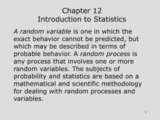
Descriptive vs Inferential • Descriptive • describe the data you’ve got • if those data are all you’re interested in, you’re done. • Inferential • make inferences about population(s) of values • (when you don’t/can’t have complete data)

Inferential • Point Estimate • Confidence Interval • Hypothesis Testing • 1 population parameter • z, t tests • 2 pop. parameters • z, t tests on differences • 3 or more?... • ANOVA!

Hypothesis Testing • Choose pop. parameter of interest • (ex: ) • Formulate null & alternative hypotheses • assume the null hyp. is true • Select test statistic (e.g., z, t) & form of sampling distribution • based on what’s known about the pop., & sample size

Defining our hypothesis • H0= the Null hypothesis • Usually designed to be the situation of no difference • The hypothesis we test. • H1= the alternative hypothesis • Usually the research related hypothesis

Null Hypothesis(~Status Quo) • Examples: • Average entering age is 28 (until shown different) • New product no different from old one (until shown better) • Experimental group is no different from control • group (until shown different) • The accused is innocent (until shown guilty)

- Ha is the hypothesis you are gathering evidence in support of. - H0 is the fallback option = the hypothesis you would like to reject. - Reject H0 only when there is lots of evidence against it. - A technicality: always include “=” in H0 - H0 (with = sign) is assumed in all mathematical calculations!!!

Decision Tree for Hypothesis Testing Test stat. n large? (CLT) Population Standard Deviation known? Pop. Distributionnormal? z-score Yes Standard normaldistribution z-score Yes Yes No No Can’t do it Yes t-score No t distribution No t-score Yes No Can’t do it

Selecting a distribution

Hypothesis Testing • Choose pop. parameter of interest • (ex: ) • Formulate null & alternative hypotheses • assume the null hyp. is true • Select test statistic (e.g., z, t) & form of sampling distribution • based on what’s known about the pop., & sample size

Hypothesis Testing • Calculate test stat.: • Note: The null hypothesis implies a certain sampling distribution • if test stat. is really unlikely under Ho, then reject Ho • HOW unlikely does it need to be? determined by 

Three equivalent methods of hypothesis testing(=significance level) p-value: prob of getting test stat at least as extreme if Ho really true.

Hypothesis Testing as a Decision Problem Great! Type II Error Power: 1 – P(Type II error) Our ability to reject the null hypothesis when it is indeed false Type I Error Great! Depends on sample size and how much the null and alternative hypotheses differ

ERRORS • Type I errors (): rejecting the null hypothesis given that it is actually true; e.g., A court finding a person guilty of a crime that they did not actually commit. • Type II errors (): failing to reject the null hypothesis given that the alternative hypothesis is actually true; e.g., A court finding a person not guilty of a crime that they did actually commit.

Type I and Type II errors Power (1-   

ANOVA: Analysis of Variance • a method of comparing 3 or more group means simultaneously to test whether the means of the corresponding populations are equal • (why not just do a bunch of 2-sample t-tests?...) • inflation of Type I error rate

ANOVA: 1-Way • You have sample data from several different groups • “One-way” refers to one factor. • Factor = a categorical variable that distinguishes the groups. • Level (group) of the factor refers to the different values that the categorical variable can take.

ANOVA: 1-Way • Examples of Factors & groups: • Factor: Political Affiliation • groups: Democrat, Republican, Independent • X=annual income • Factor: Studying Method • groups: Re-read notes, practice test, do nothing (control) • X=score on exam

ANOVA: 1-Way • So you’ve got 3(+) sets of sample data, from 3 different populations. • You want to test whether those 3 populations all have the same mean () • Null Hypothesis: • H0:1=2=3 (all pop. means are same) • H1: all pop. means are NOT the same! • [draw examples on chalkboard]

ANOVA: Assumptions • Normality • populations are normally distributed • Homogeneity of variance • populations have same variance (2) • 1-Way “Independent Samples”: • groups are independent of each other

ANOVA: the idea • Two ways to estimate 2 • MSB: Mean Square Between Group (aka MSE: MS Error) • based on how spread out the sample means are from each other. • Variation Between Samples • MSW: Mean Square Within Group • based on the spread of data within each group • Variation within Samples • If the 3(+) populations really do have same mean, then these 2 #s should be ~ the same • If NOT, then MSB should be bigger.

ANOVA: calculating • MSB: Variation between samples • (sample size) * (variance of sample means) • if sample sizes are the same in all groups • note: use the “sample variance” formula • MSW: Variation within samples • (mean of sample variances)

ANOVA: the F statistic • So how to compare MSB and MSW? • Under H0: F≈1 • So calculate your F test statistic and compare to F distribution, see if it falls in region of rejection. [chalkboard] • note: F one-tailed!

ANOVA: F & df • F distribution requires specification of 2 degrees of freedom values • DFn: degrees of freedom numerator: • (# of groups) - 1 • DFd: degrees of freedom denominator: • (total sample size (N)) - (# of groups)

ANOVA: example • Groups: adults w/ 3 different activity levels • X=% REM sleep • MSB=(sample size)(variance of sample means)=... • MSW=(mean of sample variance)=... • F=MSB/MSW=... • dfn=# groups - 1=... dfd=Ntotal-#groups=... • Fcritical=... p-value=...

Psyc 235: Introduction to Statistics