Mechanisms of enzyme inhibition

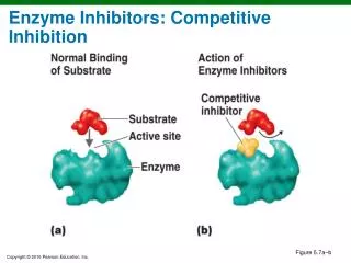
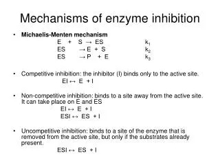
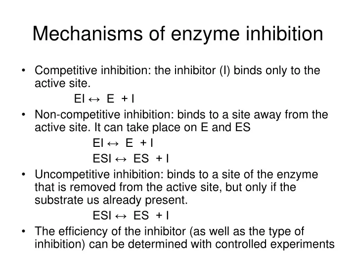
1. Mechanisms of enzyme inhibition • Competitive inhibition: the inhibitor (I) binds only to the active site. EI ↔ E + I • Non-competitive inhibition: binds to a site away from the active site. It can take place on E and ES EI ↔ E + I ESI ↔ ES + I • Uncompetitive inhibition: binds to a site of the enzyme that is removed from the active site, but only if the substrate us already present. ESI ↔ ES + I • The efficiency of the inhibitor (as well as the type of inhibition) can be determined with controlled experiments

3. Lineweaver–Burk plots characteristic of the three major modes of enzyme inhibition: • (a) competitive inhibition, • (b) uncompetitive inhibition, and • (c) non-competitive inhibition, showing the special case α = α′ > 1.

4. Autocatalysis • Autocatalysis: the catalysis of a reaction by its products A + P → 2P The rate law is = k[A][P] To find the integrated solution for the above differential equation, it is convenient to use the following notations [A] = [A]0 - x; [P] = [P]0 + x One gets = k([A]0 - x)( [P]0 + x) integrating the above ODE by using the following relation gives or rearrange into with a=([A]0 + [P]0)k and b = [P]0/[A]0

5. 23.7 Kinetics of photochemical reactions • Primary photochemical process: products are formed directly from the excited state of a reactant. • Secondary photochemical process: intermediates are formed directly from the excited state of a reactant. • Photophysical processes compete with the formation of photochemical products via deactivating the excited state

6. Times scales of photophysical processes Within 10-16 ~ 10-15 s for electronic transitions induced by radiation and thus the upper limit for the rate constant of a first order photochemical reaction is about 1016 s-1. 10-12 ~ 10-6s for fluorescence 10-12 ~ 10-4s for intersystem crossing (ISC) 10-6 ~ 10-1s for phosphorescence (large organic molecules) • A slowly decaying excited species can undergo a very large number of collisions with other reactants before deactivation. • The interplay between reaction rates and excited state lifetimes is a very important factor in the determination of the kinetic feasibility of a photochemical process.

8. The primary quantum yield, φ, the number of photophysical or photochemical events that lead to primary products divided by the number of photons absorbed by the molecules in the same time interval, or the radiation-induced primary events divided by the rate of photo absorption. • The sum of primary quantum yields for all photophysical and photochemical events must be equal to 1

10. From the above relationship, the primary quantum yield may be determined directly from the experimental rates of ALL photophysical and photochemical processes that deactivate the excited state.

11. Decay mechanism of excited singlet state • Absorption: S + hvi → S* vabs = Iabs • Fluorescence: S* → S + hvivf = kf[S*] • Internal conversion: S* → S vIC = kIC[S*] • Intersystem crossing: S* → T* vISC = kISC[S*] S* is an excited singlet state, and T* is an excited triplet state. The rate of decay = - kf[S*] - kIC[S*] - kISC[S*] • When the incident light is turn off, the excited state decays exponentially: with

12. If the incident light intensity is high and the absorbance of the sample is low, we may invoke the steady state approximation for [S*]: Iabs - kf[S*] - kIC[S*] - kISC[S*] = 0 Consequently, Iabs = kf[S*] + kIC[S*] + kISC[S*] The expression for the quantum yield of fluorescence becomes: • The above equation can be applied to calculate the fluorescence rate constant.

13. Quenching • The presence of a quencher, Q, opens an additional channel for the deactivation of S* S* + Q → S + Q vQ = kQ[Q][S*] Now the steady state approximation for [S*] gives: Iabs - kf[S*] - kIC[S*] - kISC[S*] - kQ[Q][S*] = 0 The fluorescence quantum yield in the presence of quencher becomes • The ratio of Φf,0/ Φf is then given by • Therefore a plot of the left-hand side of the above equation against [Q] should produce a straight line with the slope τ0kQ. Such a plot is called Stern-Volmer plot.

14. The fluorescence intensity and lifetime are both proportional to the fluorescence quantum yield, plot of If,0/I0 and τ0/ τ against [Q] should also be linear with the same slope and intercept as • Self-test 23.4 The quenching of tryptophan fluorescence by dissolved O2 gas was monitored by measuring emission lifetimes at 348 nm in aqueous solutions. Determine the quenching rate constant for this process [O2]/(10-2 M) 0 2.3 5.5 8 10.8 Tau/(10-9 s) 2.6 1.5 0.92 0.71 0.57

15. Three common mechanisms for bimolecular quenching 1. Collisional deactivation: S* + Q → S + Q is particularly efficient when Q is a heavy species such as iodide ion. 2. Resonance energy transfer: S* + Q → S + Q* 3. Electron transfer: S* + Q → S+ + Q- or S* + Q → S- + Q+