Download
1 / 30
300 likes | 401 Views
Chapter 5 Review. Probability – the relative likelihood of occurrence of any given outcome or event, ranges from 0 to 1 Converse Rule (not) Multiplication Rule (and) Addition Rule (or ) Z Scores – Indicates direction and degree that any raw score deviates from the mean in sigma units

E N D
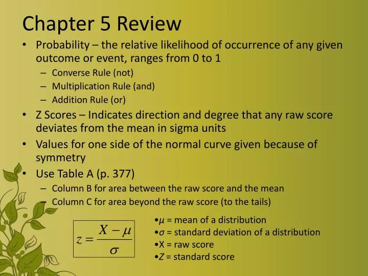
Chapter 5 Review • Probability – the relative likelihood of occurrence of any given outcome or event, ranges from 0 to 1 • Converse Rule (not) • Multiplication Rule (and) • Addition Rule (or) • Z Scores – Indicates direction and degree that any raw score deviates from the mean in sigma units • Values for one side of the normal curve given because of symmetry • Use Table A (p. 377) • Column B for area between the raw score and the mean • Column C for area beyond the raw score (to the tails) • µ = mean of a distribution • σ= standard deviation of a distribution • X = raw score • Z = standard score
Probability There are 10 people randomly selected: 7 males and 3 females. Assume that 60% of the population has brown hair, 25% has black hair, and 15% has a different color; “other.” • What is the probability that we will select... • a male? – a male with black hair? • not a female? – a female with brown hair? • two males? – a female w/brown hair or a female • one of each gender? w/black hair? • two females? – a male w/brown hair and a male w/black hair? • a male w/brown hair and not a . female w/brown hair?
Probability: Mean 28; StdDev 4 16 20 24 28 32 36 40
Introduction • Often, there is no capacity to measure an entire population • We are limited by time, energy, and economic resources • Sampling allows researchers to generalize to the wider population and has become an integral part of social science research
Samples and Populations • Population: • Set of individuals who share at least one characteristic • Sample: • A smaller number of individuals from the population that share one or more given characteristics
Sampling Methods • Researchers want to make inferences from data. • Sampling methods vary according to population and access. • Two types of sampling methods: • Non-random samples • Random samples
Sampling Error • Mean of a sample shown as • Mean of a population shown as µ • Standard deviation of a sample shown as s • Standard deviation of a population shown as σ • Mean or standard deviation of a sample rarely identical to the population • This difference is known as sampling error.
Table 1: A population and three random samples of final exam grades N = 20
Sampling Distributions of Means 96 93 92 98 96 100 106 102 105 103 99 107 101 91 102 108 95 104 Figure 1: The Mean Long Distance Phone Time in 100 Random Samples in Which the Mean = 99.75 min
Characteristics of a Sampling Distribution of Means • The sampling distribution of means approximates a normal curve. • The mean of a sampling distribution of means (the mean of means) is equal to the true population mean. • The standard deviation of a sampling distribution of means is smaller than the standard deviation of the population. -The sample mean is more stable than the scores that comprise it.
Standard Error of the Mean • Standard deviation of theoretical sampling distribution can be derived. • This is known as the standard error of the mean. • Formula for standard error of the mean: • We can now calculate the range of mean values in which our population mean is likely to fall.
Standard Error of Mean • Obtained by dividing the population standard deviation by the square root of the sample size • Illustration: IQ test • Population mean of 100 • Population standard deviation of 15 • If we took a sample of 10, subject to a standard error of? • With the aid of the standard error of the mean, we can find the range of mean values within which our true population mean is likely to fall.
Confidence Interval Cont. • Can be constructed for any level of probability • It is has become a matter of convention to use a wider, less precise confidence interval having a better probability of making an accurate or true estimate of the population mean. • 68% confidence interval = ± (1) • 95% confidence interval = ± (1.96) • 99% confidence interval = ± (2.58)
Confidence Interval Cont. • How do we go about finding the 95% confidence interval? • We already know that roughly 95% of the sample means in a sampling distribution lie between -2 standard deviations and +2 standard deviations from the mean of means. • Going to Table A, we can make the statement that 1.96 standard errors in both directions cover exactly 95% of the sample means (47.50% on either side of the mean of means). • Plus/Minus 1.96 • If we apply the 95% confidence interval to our estimate of the mean IQ of a student body, we see that 95% confidence interval = 105 +- (1.96)(3) = 105 + - 5.88 = 99.12 to 110.88
Confidence Interval Cont. • An even more stringent confidence interval is the 99% confidence interval. • From Table A, we see that the z scores 2.58 represents 49.50% of the area on either side of the curve. • Doubling this amount yields 99% of the area under the curve; • 99% of the sample means fall into this interval • By formula: • 99% confidence interval • = Sample Mean + - 2.58 standard error of the sample mean
95% Confidence Interval Using z • Suppose we want to determine the expected miles per gallon for a new Ford Explorer? • Standard deviation = 4 miles/gallon • N = 100 cars • Sample Mean = 26 miles/gallon • How do we obtain a 95% confidence interval for the mean miles/gallon for all cars of this model? • Step 1: Obtain the mean for a random sample • Step 2: Calculate the standard error of the mean • Step 3: Compute the margin of error • Step 4: Add and subtract the margin of error from the sample mean
99% Confidence Interval Using z • Now, the statistician is informed that 95% confidence is not confident enough for their needs. To be confident, we want 99%. • Standard deviation = 4 miles/gallon • N = 100 cars • Sample Mean = 26 miles/gallon • Step 1: Obtain the mean for a random sample • Step 2: Calculate the standard error of the mean • Step 3: Compute the margin of error • Step 4: Add and subtract the margin of error from the sample mean
The t ratio • Very few situations in which the population standard deviation (and thus the standard error of the mean) is known • When the exact standard deviation of the population (σ) is unknown, the t-distribution is used • Recall that sample means (and their standard deviations) are lower and more stable than population means • It is then necessary to inflate the sample standard deviation to produce more accurate estimates • Standard Error for a t ratio
Degrees of Freedom • The greater the degrees of freedom, the larger the sample size and the closer the t distribution gets to the normal distribution • df = N – 1 • Recall that the only difference between a t and a z is that the former uses an estimate of the standard error based on sample data while the latter is known
Cont. • What would one do for larger samples for which the degrees of freedom may not appear in Table B? • A sample size of 50 produces 49 degrees of freedom • t value for 49 df and alpha = .05 • 40 df = 2.021 • 60 df = 2.000 • Use the fewer degrees of freedom (ie, 40) • CI = Sample mean +/- the T value multiplied by the standard error CI = ± t*sx
The t ratio • For t-distributions, use Table C instead of Table A • Various levels of alpha • Alpha = area in the tails of the t distribution • For a 95% level of confidence, an alpha = .05. • For a 99% level of confidence, an alpha = .01. • With the addition of alpha, we now have two pieces of information available and can now construct our confidence interval • Degrees of freedom (N – 1) • Alpha value (95% = .05 or 99% = .01)Example: Construct a 95% CI with an N = 20, mean = 40
Confidence Intervals • Probability that our population mean actually falls within the range of mean values (within which our true population mean is likely to fall) • Can be constructed for any level of probability • It is has become a matter of convention to use a wider, less precise confidence interval having a better probability of making an accurate or true estimate of the population mean.
An Illustration Suppose that a researcher wanted to examine the extent of cooperation among kindergarten children. To do so, she unobtrusively observes 9 children at play for 30 minutes and notes the number of cooperative acts engaged in by each child: The mean number of cooperative acts was 2.67 and the standard deviation was 1.32. Step 1: Obtain the estimated standard error of the mean Step 2: Determine the value of t from Table C Step 3: Obtain the margin of error by multiplying the standard error of the mean by the t-ratio Step 4: Add/Subtract this product from the sample mean to find the interval within which we are 95% confident the population mean falls
Estimating Proportions • We can also estimate population proportions. • Pattern of formulas is the same. • sP= standard error of the proportion • P = sample proportion • N = total number in the sample We either use: 95% CI = P +/- 1.96*spor99% CI = P +/- 2.58*sp
An Illustration • Suppose a polling organization contacted 400 members of a local police union and asked them whether they intended to vote for candidate A or candidate B. Suppose that 55% reported their intention to vote for candidate A. Find the 95% confidence interval for candidate A. Step 1: Obtain the standard error of the proportion. Step 2: Multiply the standard error of the proportion by 1.96 to obtain the margin of error. Step 3: Add and subtract the margin of error to find the confidence interval.
Summary • Researchers rarely work with entire populations. • Sampling is necessary. • Sampling errors occur normally. • Mean of sampling means equals true population mean. • We can estimate standard deviation of sampling distribution of means. • Confidence intervals for means (or proportions) • t distributions introduced