Download
1 / 1
30 likes | 179 Views
Data assimilation in fluid dynamics. PhD Candidate: Iliass Azijli Department : AWEP Section: Aerodynamics Supervisor: R.P. Dwight Promoter: H. Bijl Start date: 01-12-2011 Funding: TNO Cooperations: TNO & IIT Madras. Raw Simulation (DNS). Raw Measurement. 1. 3. 4. 2.

E N D
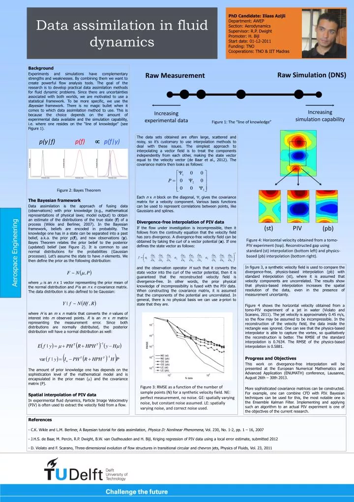
Data assimilation in fluid dynamics PhD Candidate: Iliass Azijli Department: AWEP Section: Aerodynamics Supervisor: R.P. Dwight Promoter: H. Bijl Start date: 01-12-2011 Funding: TNO Cooperations: TNO & IIT Madras Raw Simulation (DNS) Raw Measurement 1 3 4 2 Increasing simulation capability Increasing experimental data • In figure 3, a synthetic velocity field is used to compare the divergence-free, physics-based interpolation (pb) with standard interpolation (st), where it is assumed that velocity components are uncorrelated. The results show that physics-based interpolation increases the spatial resolution of the data, even in the presence of measurement uncertainty. • Figure 4 shows the horizontal velocity obtained from a tomo-PIV experiment of a jet in water (Violato and Scarano, 2011). The jet velocity is approximately 0.45 m/s, so the flow may be assumed to be incompressible. In the reconstruction of the velocity field, the data inside the rectangle was ignored. One can see that the physics-based interpolator is able to capture the vortex, so qualitatively the reconstruction is better. The RMSE of the standard interpolation is 0.7634. The RMSE of the physics-based interpolation is 0.5881. • Progress and Objectives • This work on divergence-free interpolation will be presented at the European Numerical Mathematics and Advanced Application (ENUMATH) conference, Lausanne, August 26th – 30th 2013. • More sophisticated covariance matrices can be constructed. For example, one can combine CFD with PIV. Bayesian techniques can be used for this, the most notable one is the Ensemble Kalman Filter. Implementing and applying such an algorithm to an actual PIV experiment is one of the objectives of the current research. • Background • Experiments and simulations have complementary strengths and weaknesses. By combining them we want to create powerful flow analysis tools. The goal of the research is to develop practical data assimilation methods for fluid dynamic problems. Since there are uncertainties associated with both worlds, we are motivated to use a statistical framework. To be more specific, we use the Bayesian framework. There is no magic bullet when it comes to which data assimilation method to use. This is because the choice depends on the amount of experimental data available and the simulation capability, i.e. where one resides on the “line of knowledge” (see Figure 1). • The Bayesian framework • Data assimilation is the approach of fusing data (observations) with prior knowledge (e.g., mathematical representations of physical laws; model output) to obtain an estimate of the distributions of the true state (f) of a process (Wikle and Berliner, 2007). In the Bayesian framework, beliefs are encoded in probability. The knowledge one has in a state can be separated into a past belief, a.k.a. the prior p(f), and new observations (y). Bayes Theorem relates the prior belief to the posterior (updated) belief (see Figure 2). It is common to use normal distributions for the probabilities (Gaussian processes). Let’s assume the state to have n elements. We then define the prior as the following distribution: • where is an n x 1 vector representing the prior mean of the normal distribution and P is an n x n covariance matrix. The data distribution is also defined to be Gaussian: • where H is an m x n matrix that converts the n values of interest into m observed points. R is an m x m matrix representing the measurement error. Since both distributions are normally distributed, the posterior distribution will have a normal distribution as well: • The amount of prior knowledge one has depends on the sophistication level of the mathematical model and is encapsulated in the prior mean () and the covariance matrix (P). • Spatial interpolation of PIV data • In experimental fluid dynamics, Particle Image Velocimetry (PIV) is often used to extract the velocity field from a flow. Figure 1: The “line of knowledge” The data sets obtained are often large, scattered and noisy, so it’s customary to use interpolation methods to deal with these issues. The simplest approach to interpolating a vector field is to treat the components independently from each other, making the state vector equal to the velocity vector (de Baar et al., 2012). The covariance matrix then looks as follows: Each n x n block on the diagonal, i gives the covariance matrix for a velocity component. Various basis functions can be used to represent correlations between points, like Gaussians and splines. Divergence-free interpolation of PIV data If the flow under investigation is incompressible, then it follows from the continuity equation that the velocity field has zero divergence. A divergence-free velocity field can be obtained by taking the curl of a vector potential (a). If one defines the state vector as follows: and the observation operator H such that it converts the state vector into the curl of the vector potential, then it is guaranteed that the reconstructed velocity field is divergence-free. In other words, the prior physical knowledge of incompressibility is fused with the PIV data. When constructing the covariance matrix, it is assumed that the components of the potential are uncorrelated. In general, there is no physical basis we can use a-priori to state that they are. Figure 2: Bayes Theorem Aerospace Engineering (st) PIV (pb) Figure 4: Horizontal velocity obtained from a tomo-PIV experiment (top). Reconstructed gap using standard (st) interpolation (bottom left) and physics-based (pb) interpolation (bottom right). p(f) p(f|y) p(y|f) Figure 3: RMSE as a function of the number of sample points (N) for a synthetic velocity field. NE: perfect measurement, no noise. GE: spatially varying noise, but constant noise assumed. LE: spatially varying noise, and correct noise used. • References • C.K. Wikle and L.M. Berliner, A Bayesian tutorial for data assimilation, Physica D: Nonlinear Phenomena, Vol. 230, No. 1-2, pp. 1 – 16, 2007 • J.H.S. de Baar, M. Percin, R.P. Dwight, B.W. van Oudheusden and H. Bijl, Kriging regression of PIV data using a local error estimate, submitted 2012 • D. Violato and F. Scarano, Three-dimensional evolution of flow structures in transitional circular and chevron jets, Physics of Fluids, Vol. 23, 2011