Download
1 / 45
450 likes | 716 Views
Course 6 動態規劃 Dynamic Programming. ▓ Outlines. 本章重點 Divide-and-Conquer v.s. Dynamic Programming Dynamic Programming v.s. Greedy Approach Floyd's Algorithm for Shortest Paths Chained Matrix Multiplication Dynamic Programming and Optimization Problems.

E N D
▓ Outlines • 本章重點 • Divide-and-Conquer v.s. Dynamic Programming • Dynamic Programming v.s. Greedy Approach • Floyd's Algorithm for Shortest Paths • Chained Matrix Multiplication • Dynamic Programming and Optimization Problems
▓ Divide-and-Conquer v.s. Dynamic Programming • 由前一單元得知,Divided-and-Conquer即為遞迴解法。 • 以費氏數 (Fibonacci Number) 說明: 終止條件 遞迴關係
Recursive Fibonacci Algorithm inputs: num identified the ordinal of the Fibonacci number outputs: returns the nth Fibonacci number void Fib(int num) { if (num is 0 OR num is 1) return num; else return (Fib(num-1) + Fib(num-2)); }
Based on recursive function, 求取Fib (8)的過程如下: • Top-Down求算方式 • 子問題重覆 (Overlapping Subproblem) 是Divided-and-Conquer主要的問題所在
以人的方式求算: • 求算F8和F7時,F6會被用到2次,但我們用表格記錄已算過的部份!! • Bottom-Up求算方式 • 動態規劃 (Dynamic Programming)是一種表格式的演算法設計原則。 • 其精神是將一個較大的問題定義為較小的子問題組合,先處理較小的問題,並將其用表格儲存起來,再進一步地以較小問題的解逐步建構出較大問題的解。 • Programming: 用表格存起來,有 “以空間換取時間”之涵意 • 屬於作業研究 (OR)的技巧
Divide-and-Conquer 和 Dynamic Programming都是將問題切割再採用遞迴方式處理子問題,但是: • Divide-and-Conquer可能會對相同子問題進行重覆計算 • Dynamic Programming會使用表格將子問題的計算結果加以儲存,在後面階段如果需要這個計算結果,再直接由表格中取出使用,因此可以避免許多重覆的計算,以提高效率。 • Divide-and-Conquer v.s. Dynamic Programming
▓ Dynamic Programming v.s. Greedy Approach • 對於具有限制的最佳化問題,可以採用 “貪婪法則” 或 “動態規劃” 來設計演算法則。 • Greedy Approach: • 是一種階段性 (Stage)的方法 • 具有一選擇程序 (Selection Procedure),自某起始點(值) 開始,在每一個階段逐一檢查每一個輸入是否適合加入答案中,重複經過多個階段後,即可順利獲得最佳解 • 較為簡單 (若遇最佳化問題,先思考可否用Greedy Approach解,若不行再考慮用Dynamic Programming) • 如果所要處理的最佳化問題無法找到一個選擇程序,則需要考慮所有的可能情況,就是屬於Dynamic Programming • Dynamic Programming • 先把所有的情況都看過一遍,才去挑出最佳的結果 • 考慮問題所有可能的情況,將最佳化問題的目標函數表示成一個遞迴關係式,結合Table的使用以找出最佳解
A 3 1 B D 2 2 4 C A A 3 3 1 1 B D B D 2 2 C C • Ex 1. 有一Graph如下,每一個邊都有一權重值,試找出 “具最小權重值總合且不包含Cycle” 的 Graph。 • Sol: (選擇程序) 從最小的邊開始逐一選擇,挑選出來的邊不能構成Cycle,直到所有的邊都被選完為止。 或
B 2 4 A D 3 2 C B 2 4 A D 3 2 C • Ex 2. 一有向加權圖Graph如下,該圖可分成2個部份,請找出由第一個部份的出發頂點到最後部份的目的地頂點的最短距離路。 • Sol: 找不到一個選擇程序,可自某起始點(值) 開始逐一檢查每一個輸入是否適合加入答案中。
▓ Floyd's Algorithm for Shortest Paths • 最短路徑 (Shortest Path) 問題 • 給定一個有向加權圖形 (Directed Weighted Graph),G=(V, E),找出任意兩個頂點(v1, v2 V) 之間的最短路徑 • All-pair Shortest Path問題 • In Figure 3.2, there are three simple paths from v1 to v3—namely [v1, v2, v3], [v1, v4, v3] and [v1, v2, v4, v3] . Because [v1, v4, v3] is the shortest path from v1 to v3.
The Shortest Paths problem is an optimization problem. • There can be more than one candidate solution to an instance of an optimization problem. • Each candidate solution has a value associated with it, and a solution to the instance is any candidate solution that has an optimal value. • Depending on the problem, the optimal value is either the minimum or the maximum. • In the case of the Shortest Paths problem, • a candidate solution is a path from one vertex to another, • the value is the length of the path, and • the optimal value is the minimum of these lengths.
6 v1 v2 4 11 2 3 v3 • 佛洛依德最短路徑演算法 (Floyd‘s Algorithm for Shortest Paths) : • Floyd-Warshall Algorithm • 假設G=(V, E),|V| = n • Dk矩陣: 為一 nn的矩陣,其中Dk[i, j]表示自 vi至 vj (vi vj )的最短路徑長,且途中經過的頂點編號均 ≤ k(其中k≥0) • 範例: D1[2, 1] = 6 2 → 1 (合法) 2 → 1 → 2 → 1 (不合法) 2 → 3 → 1 (不合法) D2[2, 1] = 6 2 → 1 (合法) 2 → 1 → 2 → 1 (合法) 2 → 3 → 1 (不合法) D3[2, 1] = 5 2 → 1 (合法) 2 → 1 → 2 → 1 (合法) 2 → 3 → 1 (合法) ∵節點個數為 3 ∴ D3[i, j]可得到總體最短路徑
6 v1 v2 4 11 2 3 v3 • 當k = 0時, 矩陣D0[i, j]表示為Adjacency Matrix (相鄰矩陣; W)。 • 自 vi至 vj途中不會經過其它頂點 • Floyd‘s Algorithm求解過程: • 找出相鄰矩陣 W • 逐步求出D1, D2, …, Dn矩陣 • Dn矩陣即為結果
6 v1 v2 4 11 2 3 v3 • 求解右圖的All-pair Shortest Path Sol: • 找出相鄰矩陣 W • 逐步求出D1, D2, D3矩陣 • Step 1: 由 W矩陣求出 D1矩陣 4 11 0 6 0 2 3 7 0
Step 2: 由 D1 矩陣求出 D2矩陣 • Step 3: 由 D2 矩陣求出 D3 矩陣 6 0 4 0 2 6 0 3 7 4 0 6 5 0 2 0 3 7
Dk-1[i, j] vi vj Dk-1[i, k] Dk-1[k, j] vk • Floyd‘s Algorithm觀念圖解: • 求矩陣Dk[i, j],是由矩陣Dk-1[i, j]而來
//k為 Dk 的k值 Time Complexity: O(n3)
-4 -1 1 1 2 2 3 3 2 3 4 4 • Floyd‘s Algorithm的假設條件: • 圖形中不得有負長度的Cycle存在 • 例 1: 1 →2的最短路徑為 - • 例 2: 1 →2的最短路徑為 3
▓ Chained Matrix Multiplication • Suppose we want to multiply a 2 × 3 matrix times a 3 × 4 matrix as follows: • The resultant matrix is a 2 × 4 matrix. • If we use the standard method of multiplying matrices, it takes three elementary multiplications to compute each item in the product. • Because there are 2 × 4 = 8 entries in the product, the total number of elementary multiplication is • In general, to multiply an i × j matrix times a j × k matrix using the standard method, it is necessary to do
Note: n個matrix相乘有 種可能的配對組合 (括號方式) • Ex: Consider the multiplication of the following four matrices: There are five different orders in which we can multiply four matrices, each possibly resulting in a different number of elementary multiplications: The third order is the optimal order for multiplying the four matrices.
Chained Matrix Multiplication: • Def: 給一Matrix Chain: A1, A2, …, An,求此Chain所需之純量積乘法次數為最少之括號方式 (即: 最佳的矩陣乘法組合方式)。 • 若Ai, Ai+1, …, Aj 在某組合方式所需的純量積乘法次數為最小 (最佳),則必存在一個k,使得Ai, Ai+1, …, Ak 和Ak+1, Ak+2, …, Aj皆為最佳。 ((Ai Ai+1 … Ak )(Ak+1 Ak+2 …, Aj)) • Matrix Chain的遞迴式 最佳組合 最佳子組合 最佳子組合
Chained Matrix Multiplication 問題的演算法需有兩個表格和一個主要變數: • M[i, j] • 記錄多個矩陣相乘 (e.g., Ai … Aj)時,所需的 “最少” 乘法次數 • P[i, j] • 記錄多個矩陣相乘 (e.g., Ai … Aj) 所需最少乘法次數之 “最佳乘法順序” 是由哪一個矩陣開始分割 • diagonal • 主要指出在Matrix Chain中,每一次有多少個矩陣要相乘 • diagonal = 1 只有1個矩陣,∴不會執行乘法動作 • diagonal = 2 每一次有2個矩陣要相乘 • diagonal = 3 每一次有3個矩陣要相乘 • diagonal = 4 每一次有4個矩陣要相乘 • …
The optimal order for multiplying six matrices must have one of these factorizations: • 第k個分解型式所需的乘法總數,為前後兩部份 (一為A1, A2, …, Ak 和Ak+1, …, A6) 各自所需乘法數目的最小值相加,再加上相乘這前後兩部份矩陣所需的乘法數目。
Matrix Chain的遞迴式 • Example: A133, A237, A372, A429, A594, 求此五矩陣的最小乘法次數。 Sol: 建立兩陣列 M[1…5, 1…5]及P[1…4, 2…5]
分割點k = 1 Case (When diagonal = 1) • diagonal = 1,∵只有1個矩陣,∴不會執行乘法動作 • 陣列M的中間對角線為0,陣列P則不填任何數值 Case (When diagonal > 1) • diagonal = 2,有2個矩陣相乘 • 當 i = 1及 j = 2,為A1及A2矩陣相乘,此時: M[1, 2] = M[1,1]+M[2,2]+337 = 63, 其中 A1 及A2 的分割點 k 如下: A1A2 diagonal = 1 diagonal = 2
Case (When diagonal > 1) • diagonal = 3,有3個矩陣相乘 • 當 i = 2及 j = i+diagnal-1 = 2+3-1=4,為A2至A4間的所有矩陣相乘,此時: diagonal = 3
Case (When diagonal > 1) • diagonal = 4,有4個矩陣 • 當 i = 1及 j = 4,為A1至A4間的所有矩陣相乘,此時: diagonal = 4
Case (When diagonal > 1) • diagonal = 5,有5個矩陣 • 當 i = 1及 j = 5,為A1至A5間所有矩陣相乘,此時: diagonal = 5
[Note]此演算法的概念如下: A1, A2, A3, A4, A5 A1A2, A2A3, A3A4, A4A5 A1A2A3, A2A3A4, A3A4A5 A1A2A3A4, A2A3A4A5 A1A2A3A4A5 diagonal = 1 diagonal = 2 diagonal = 3 diagonal = 4 diagonal = 5
Case (When diagonal > 1) Case (When diagonal > 1)
▓ Dynamic Programming and Optimization Problems • Dynamic Programming 和 Greedy Approach看似可以處理所有的最佳化問題,然而它們所能處理的最佳化問題需滿足下列原則 • Definition: The principle of optimality (最佳化原則) is said to apply in a problem if an optimal solution to an instance of a problem optimal solutions to all substances. (當一個問題存在著最佳解,則表示其所有子問題也必存在著最佳解) • In the case of the Shortest Paths problem we showed that if vk is a vertex on an optimal path form vi to vj , then the subpaths from vi to vk and from vk to vj must also be optimal.
每一個輸入的計算都必須是根據其餘輸入的最佳結果再進一步計算,如此才能夠得到最佳解,同時可以將無法獲得最佳解的情況去除,以避免需要將每一種可能情況都加以考慮。每一個輸入的計算都必須是根據其餘輸入的最佳結果再進一步計算,如此才能夠得到最佳解,同時可以將無法獲得最佳解的情況去除,以避免需要將每一種可能情況都加以考慮。 • 對於n個輸入的最佳化問題 (X1, X2, …, Xn): • 有些被歸類為 “部份集合” (Subset) 問題,會有2n種可能的情況 • 有些被歸類為 “排列組合” (Permutation) 問題,會有n!種可能的情況 • 因此皆屬指數複雜度的問題,若可採用最佳化原則通常可以將這一些問題的複雜度由指數複雜度降為多項式複雜度。 • 然而,並不是所有求最佳化的問題都合乎最佳化原則,此時就只能用其它的方法求解了。
The Pairwise Sequence Alignment • Compare two sequence • Some reasons to perform the sequence alignment operations • Measure the similarity of two sequences. • A DNA sequence X and a database containing a set of DNA sequences. • Data compression.
String v.s. Sequence • String • a segment of consecutive characters. • usually called sequence in Biology. • Sequence • need not be consecutive. • Example: • S = “a t g a t g c a a t” • Substrings of S: “g a t g c”, “t g c a a t”. • Subsequences of S: “a g g t”, “a a a a”. • In Biology, String → Sequence.
S1 G A A C T G --- --- --- S1 G A A C T G S2 G A --- --- --- G C T G S2 G A G C T G 2 +2 -1 +2 +2 +2 2 +2 -1 -1 -1 +2 -1 -1 -1 Score=9 Score=0 • We have two sequences S1 and S2: • A scoring rule to measure the goodness of an alignment: • ai=bj, Score=2 • ai or bj align with a blank, Score=-1 • ai≠bj, Score=-1 Better
--- --- G C G S1 G A T S2 G A A C T G --- --- Sequence A: GAACTG Sequence B: GAGCTG An alignment of A and B: Mismatch Match Insertion gap Deletion gap
G A G C T G GAACTG --- --- G C G S1 G A T S2 G A A C T G --- --- S1 S2
6 -2 -3 -4 -5 -6 b c 5 4 3 2 1 b d a -1 a S1 a b b c a d S2 e a c b i 0 ai j 0 bj -1 -2 -3 -4 -5 -6 1 e -1 1 0 -1 -2 -2 -3 2 a -2 0 0 -1 1 0 -1 3 c -3 -1 2 2 1 0 -1 4 b -4 • Find an alignment which has the highest score. 0 A(i,j)=the score of optimal alignment A(0,0)=0 A(i,0)= -i A(0,j)= -j If ai=bj, then A(i,j)= A(i-1,j-1) +2 Else A(i,j)=Max(A(i-1,j) –1, A(i,j-1) –1, A(i-1,j-1) –1 )
0 -1 5 4 -1 -3 -4 -5 -6 c -2 b a a d 1 6 2 b 3 1 0 -1 S1 a b b c a d S2 e a c b 0 i 0 1 0 - a b b c a d j -1 0 0 e a c b - - - 1 0 -1 1 e -1 -1 -2 -3 -4 -5 -6 - a b b c a d 1 e a - - c b - 2 a -2 1 0 -1 -2 -2 -3 0 - a b b c a d 3 c -3 0 0 -1 1 0 -1 e a - - c - b 4 b -4 -1 2 2 1 0 -1 0 -1 1 0 1 0 -1 2 Tracing back the table