Download
1 / 41
430 likes | 573 Views
Digital Sound as Computer Science. Jennifer Burg. CPATH Workshop Series: “Revitalizing Computer Science Education Through the Science of Digital Media” Workshop 2, July 28 and 29, 2008 Wake Forest University.

E N D
Digital Sound as Computer Science Jennifer Burg CPATH Workshop Series: “Revitalizing Computer Science Education Through the Science of Digital Media” Workshop 2, July 28 and 29, 2008 Wake Forest University This work was funded by National Science Foundation CPATH grant CCF 0722261, Jennifer Burg PI, Conrad Gleber Co-PI
National Science Foundation CPATH Grant • “Revitalizing Computer Science Education through the Science of Digital Media” • Jennifer Burg, PI, Wake Forest University • Conrad Gleber, Co-PI, La Salle University • Three years (Aug. 2007 – July 2010), seven workshops • Each workshop • A special digital media topic • One speaker from a related academic discipline • One speaker from a related business or industry • What would they like to see in a computer science major working for or with them?
Digital Sound Production Workshop • June 2 to July 25, 2008 • Students of music and computer science working together • Interdisciplinary collaborative projects • Funded by National Science Foundation CCLI grant “Linking Science, Art, and Practice through Digital Sound,” Jennifer Burg, PI; Jason Romney, Co-PI
Goals in this workshop from the PIs’ perspective • Consider in what ways digital sound is legitimately part of the computer science curriculum • Explore concepts, assignments, experiments, and exercises that are interesting to students because they bring together science, art, and practice • Figure out where these can be plugged into the computer science curriculum
Goals in this workshop from the participants’ perspective • Consider how these ideas shed light on your own work • Make contacts with colleagues who share your interests • Eat well
What does the study of digital sound entail? • Physics • sound waves, acoustics, resonance • Engineering and digital signal processing (DSP) • Sound card, microphones, speakers, hardware sound processors, cables • Mathematics • Trigonometry, logarithms, complex numbers, summations, integrals, transforms • Music • Fundamental frequencies, harmonics, octaves • Algorithms • Transforms, filters, compression
What makes digital sound a suitable topic within computer science? • It’s based on digital encoding and manipulation of digital data. • It’s “applied” computer science, which is what makes it interesting.
Topics in Digital Sound as Computer Science • Sound waves and acoustics • Analog vs. digital representations, digital encoding, sampling and quantization • Decibels for measuring amplitude • Frequencies related to pitch, complex waveforms • Implications of sampling rate: the Nyquist theorem and aliasing • Implications of bit depth: quantization error, SQNR, dynamic range, dithering, noise shaping, dynamic compression and expansion
Topics in Digital Sound as Computer Science • MIDI compared to digital audio • MIDI message formats and protocols • MIDI samplers vs. synthesizers • Sound wave synthesis
Topics in Digital Sound as Computer Science • Hardware for sound processing • Sound cards; ADCs and DACs; connection types; cables; microphones, speakers and monitors; frequency response of microphones, speakers, and monitors • Software for sound processing • Audition, Audacity, Sound Forge, Logic, Pro Tools, Reason, Cakewalk Music Creator and Sonar, etc. • MATLAB • Chuck
Topics in Digital Sound as Computer Science • Fourier analysis, frequency components, the Fourier transform, windowing functions • Filters (FIR and IIR), EQ, types of filters (shelf, low-pass, high-pass, bandpass, bandstop) • Special effects, e.g. reverb, autotuning, vocoding • Data rate, data compression, psychoacoustical models for compression, frequency masking
As is true with most topics in computer science, you can approach digital sound at different levels of abstraction • Mathematical/algorithmic – pencil and paper, chalkboard, and calculator • Low-level programming (e.g. C under Linux) • Chuck • MATLAB • Audition, Audacity, Sound Forge, Logic, Pro Tools, Reason, various plugins, etc. • Sample editor vs. track editor • Combining digital audio and MIDI
Frequency Components of Sound Waves • Generate notes C4, E4, and G4. Add the waves and look at the result. • In Audition • In MATLAB • A single-frequency wave is a single pitch. • Voices and instruments don’t produce single pitches. They have harmonics. • Sound in music and nature are complex waveforms with frequency components.
Notes, Octaves, and Frequencies • Let f1 and f2 be the frequencies of two notes where the second is an octave above the first. Then f2 = 2*f1. • There are 12 notes in an octave. Find x such that • f2 =2*f1 = ((((((((((((f1*x)*x)*x)*x)*x)*x)*x)*x)*x)*x)*x)*x) • 2*f1= f1*x12 • 2 = x12 • x = 1.0595 • Thus if fa and fb are the frequencies of two consecutive notes, then fb = 1.0595 * fa.
Nyquist Theorem and Aliasing • The sampling rate must be more than twice the frequency of the highest frequency component of the sound being sampled. • Otherwise you can have aliasing. • A frequency component comes out lower than it should be. • Demonstrated in Audition
How is amplitude measured? In Audition
The Effect of Bit Depth in Quantization • Rounding to discrete quantization levels causes error. The error is itself a wave. • In MATLAB • Signal to quantization noise ratio (SQNR) and dynamic range are also measured in decibels.
Audio Dithering • Add a random amount between -1 and 1 (scaled to the bit depth of the audio file) to each sample before quantizing. • There will be fewer consecutive samples that round to the same amount. Rounding to 0 is the worst thing, causing breaks. • Demonstration • In Audition • In MATLAB
Noise Shaping • Raise error wave above the Nyquist frequency. • Do this by making the error go up if it was previously down and down if it was previously up. This raises the error wave’s frequency. • The amount added to a sample depends on the error in previous sample.
Digital Filters • Infinite impulse response (IIR) vs. finite impulse response (FIR) filters • Filtering in the time domain by means of convolution Click to animate
Digital Filters • Filtering in the frequency domain by means of the Fourier transform
Creating Filters frequency response graph
Creating Filters frequency response graphs
Creating a Low-Pass Filter Frequency Response (frequency domain) Impulse Response (time Domain)
Creating a Low-Pass Filter • You can do it yourself in MATLAB: • Create the filter using the given function, sin(2fc)/n • Read in an audio clip • Since this is a filter in the time domain, convolve audio clip with the filter • Listen to the result • Graph the frequencies of filtered clip against the unfiltered clip. (Do this by taking the Fourier transform of each first.) • See the demonstration and worksheet for details.
Creating FIR and IIR Filters with MATLAB’s Digital Signal Processing Toolbox >> lowA = wavread('440.wav'); >> highA = wavread('880.wav'); >> highest = wavread('2000.wav'); >> mixed = (lowA+highA+highest) / 3; >> [a,b] = butter(6,1000/4000); >> output = filter(a,b,mixed); >> ideal = (lowA+highA) / 2; >> wavplay(ideal,8000); >> wavplay(output,8000); >> hold on >> plot(ideal); >> plot(output,'red'); >> axis([1 50 -1 1]) Demonstration
Filter Visualization Tool in MATLAB • MATLAB also has a Filter Visualization Tool that lets you set zeros and poles for a filter and see the frequency, phase, and impulse responses. Demonstration
C Programs for Digital Sound and MIDI Reading Messages from dev/midi #include <stdio.h> #include <string.h> #include <linux/soundcard.h> #include <unistd.h> #include <fcntl.h> /*CTRL-Break out of program*/ int main() { char* device00 = "/dev/midi" ; unsigned char data[3]; unsigned char byte1, byte2, byte3; int fd fd = open(device00, O_RDONLY, 0); if (fd < 0) { printf("Error: cannot open %s\n", device00); } else printf("Opened dev/midi00\n"); byte1 = byte2 = byte3 = -1; while (1) { read(fd, data, sizeof(data)); if (!(data[0] == byte1 && data[1] == byte2 && data[2] == byte3) { printf("%d ", data[0]); printf("%d ", data[1]); printf("%d\n", data[2]); byte1 = data[0]; byte2 = data[1]; byte3 = data[2]; } } return 0; }
Reading from and Writing to the Sound Card #include <unistd.h> #include <fcntl.h> #include <sys/types.h> #include <sys/ioctl.h> #include <stdlib.h> #include <stdio.h> #include <linux/soundcard.h> #define LENGTH 3 #define RATE 8000 #define SIZE 8 #define CHANNELS 1 unsigned char buf[4*LENGTH*RATE*SIZE*CHANNELS/8]; int main(){ int fd, arg, status; int i, j, k, begin, end, bufEnd; char temp; printf("Size of buffer is %d\n", sizeof(buf)); fd = open("/dev/dsp", O_RDWR, 0); if (fd < 0) { perror("Opening /dev/dsp failed\n"); exit(1); } arg = SIZE; status = ioctl(fd, SOUND_PCM_WRITE_BITS, &arg); if (status == -1) perror("Unable to set sample size\n");
Reading from and Writing to the Sound Card arg = CHANNELS; status = ioctl(fd, SOUND_PCM_WRITE_CHANNELS, &arg); if (status == -1) perror("Unable to set number of channels\n"); arg = RATE; status = ioctl(fd, SOUND_PCM_WRITE_RATE, &arg); if (status == -1) perror("Unable to set sampling rate\n"); status = read(fd, buf, 1); while (buf[0] >= 125 && buf[0] <= 131) { status = read(fd, buf, 1); } printf("%d ",buf[0]); printf("broke the silence\n");
Reading from and Writing to the Sound Card for (i = 0; i <= 3; i++) { //printf("Say something\n"); status = read(fd, buf+(24000*i), 24000); if (status != 24000) perror("Read wrong number of bytes\n"); begin = 24000*i; end = begin + 12000; bufEnd = begin + 24000 - 1; for (j = begin, k = 0; j < end; j++, k++) { temp = *(buf+j); *(buf+j) = *(buf + bufEnd - k); *(buf+j) = temp; } } status = ioctl(fd, SOUND_PCM_SYNC, 0); if (status == -1) perror("SOUND_PCM_SYNC failed\n"); printf("You said \n"); status = write(fd, buf, sizeof(buf)); if (status != sizeof(buf)) perror("Wrote wrong number of bytes\n"); }
Creating a Vocoder in MATLAB From http://www.paia.com/ProdArticles/vocodwrk.htm
Creating a Vocoder in MATLAB function output = vocoder(input1, input2, s, window) h = hanning(window)'; input1 = input1'; input2 = input2'; q=(s-window); output = zeros(1,s); fftdata = zeros(1,s); input1fft = zeros(1,s); input2fft = zeros(1,s); for i=1:window/4:q b = i+window-1; input1partfft = fft(input1(i:b).*h); input2partfft = fft(input2(i:b).*h); input1fft(i:b) = input1fft(i:b) + abs(input1partfft); input2fft(i:b) = input2fft(i:b) + abs(input2partfft); mult = input1partfft.*input2partfft; fftdata(i:b) = fftdata(i:b)+ abs(fft(mult)); output(i:b) = output(i:b)+ifft(mult); end output = output/max(output); Demonstration
Questions for this workshop • How do we relate the science to art and practice? • How much science does the artist/practitioner need? • Where are the points where knowing the science results in better work? • How do we change the computer science curriculum to retain the science but relate it more interestingly to art and practice?