INTRODUCTION

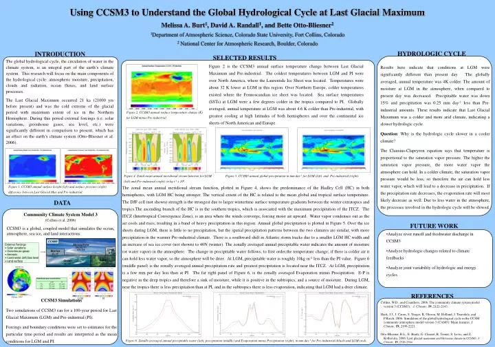
1. Atmosphere T85,T42,T31 2.8 x 2.8 Sea Ice x1°,x3° Land T85,T42,T31 Using CCSM3 to Understand the Global Hydrological Cycle at Last Glacial MaximumMelissa A. Burt1, David A. Randall1, and Bette Otto-Bliesner21Department of Atmospheric Science, Colorado State University, Fort Collins, Colorado2 National Center for Atmospheric Research, Boulder, Colorado HYDROLOGIC CYCLE INTRODUCTION SELECTED RESULTS The global hydrological cycle, the circulation of water in the climate system, is an integral part of the earth’s climate system. This research will focus on the main components of the hydrological cycle: atmospheric moisture, precipitation, clouds and radiation, ocean fluxes, and land surface processes. The Last Glacial Maximum occurred 21 ka (21000 yrs before present) and was the cold extreme of the glacial period with maximum extent of ice in the Northern Hemisphere. During this period external forcings (i.e. solar variations, greenhouse gases, sea level, etc.) were significantly different in comparison to present, which has an effect on the earth’s climate system (Otto-Bliesner et al. 2006). Figure 2 is the CCSM3 annual surface temperature change between Last Glacial Maximum and Pre-industrial. The coldest temperatures between LGM and PI were over North America, where the Laurentide Ice Sheet was located. Temperatures were about 32 K lower at LGM in this region. Over Northern Europe, colder temperatures existed where the Fennoscandian ice sheet was located. Sea surface temperatures (SSTs) at LGM were a few degrees colder in the tropics compared to PI. Globally averaged, annual temperature at LGM was about 4.6 K colder than Pre-industrial, with greatest cooling at high latitudes of both hemispheres and over the continental ice sheets of North American and Europe. Results here indicate that conditions at LGM were significantly different than present day. The globally averaged, annual temperature was 4K colder. The amount of moisture at LGM in the atmosphere, when compared to present day was decreased. Precipitable water was down 15% and precipitation was 0.25 mm day-1 less than Pre-industrial amounts. These results indicate that Last Glacial Maximum was a colder and more arid climate, indicating a slower hydrologic cycle. Question: Why is the hydrologic cycle slower in a cooler climate? The Clausius-Clapeyron equation says that temperature is proportional to the saturation vapor pressure. The higher the saturation vapor pressure, the more water vapor the atmosphere can hold. In a colder climate, the saturation vapor pressure would be less, so therefore the air can hold less water vapor, which will lead to a decrease in precipitation. If the precipitation rate decreases, the evaporation rate will most likely decrease as well. Due to less water in the atmosphere, the processes involved in the hydrologic cycle will be slowed. Figure 2. CCSM3 annual surface temperature change (K) for LGM minus Pre-industrial. Figure 4. Zonal mean annual meridional stream function for LGM (left) and Pre-industrial (right), in kg s-1 x 106. Figure 5. CCSM3 annual global precipitation in mm day-1 for LGM (left) and Pre-industrial (right). Figure 1. CCSM3 annual surface height (left) and surface pressure (right) difference between Last Glacial Max and Pre-industrial. The zonal mean annual meridional stream function, plotted in Figure 4, shows the predominance of the Hadley Cell (HC) in both hemispheres, with LGM HC being stronger. The vertical extent of the HC is related to the mean global and tropical surface temperature. The DJF cell (not shown) strength is the strongest due to larger wintertime surface temperature gradients between the winter extratopics and tropics.The ascending branch of the HC is in the southern tropics, which is associated with the maximum precipitation of the ITCZ. The ITCZ (Intertropical Convergence Zone), is an area where the winds converge, forcing moist air upward. Water vapor condenses out as the air cools and rises, resulting in a band of heavy precipitation in this region. Annual global precipitation is plotted in Figure 5. Over the ice sheets during LGM, there is little to no precipitation, but the spatial precipitation patterns between the two climates are similar, with more precipitation in the warmer Pre-industrial climate. There is a southward shift in Atlantic storm tracks due to a smaller LGM HC width and an increase of sea ice cover (not shown) to 40N (winter). The zonally averaged annual precipitable water indicates the amount of moisture (or water vapor) in the atmosphere. The change in precipitable water follows, to first order,the temperature change; if there is colder air it can hold less water vapor, so the atmosphere will be drier. At LGM, precipitable water is roughly 10kg m-2 less than the PI value. Figure 6 (middle panel) is the zonally averaged annual precipitation rate and greatest precipitation is located near the ITCZ. At LGM, precipitation is a few mm per day less than at PI. The far right panel of Figure 6, is the zonally averaged Evaporation minus Precipitation. E-P is negative in the deep tropics and therefore a sink of moisture, while it is positive in the subtropics, and a source of moisture. During LGM, near the tropics there is less precipitation than at PI, and in the subtropics there is less evaporation, indicating that LGM had a drier climate. DATA Community Climate System Model 3 (Collins et al. 2006) CCSM3 is a global, coupled model that simulates the ocean, atmosphere, sea ice, and land interactions. FUTURE WORK • Analyze river runoff and freshwater discharge in CCSM3 • Analyze hydrologic changes related to climate feedbacks • Analyze joint variability of hydrologic and energy cycles CCSM3 External Forcings • Solar variations • Greenhouse gases • Aerosols • Continental drift/Sea level • Land surface Land Ice Land Ice Ocean x1°, x3° REFERENCES Peltier 2004 LGM PI CCSM3 Simulations Two simulations of CCSM3 ran for a 100-year period for Last Glacial Maximum (LGM) and Pre-industrial (PI). Forcings and boundary conditions were set to estimates for the particular time period and results are interpreted as the mean conditions for LGM and PI. Collins, W.D., and Coauthors, 2006: The community climate system model version 3 (CCSM3). J. Climate, 19, 2122-2143. Hack, J.J., J. Caron, S. Yeager, K. Oleson, M. Holland, J. Truesdale, and P.Rasch, 2006: Simulation of the global hydrological cycle in the CCSM community atmosphere model version 3 (CAM3): Mean features. J. Climate, 19, 2199-2221. Otto-Bliesner, B.L., E. Brady, G. Clauzet, R. Tomas, S. Levis, and Z. Kothavala, 2006: Last glacial maximum and Holocene climate in CCSM3. J. Climate, 19, 2526-2544. Figure 6. Zonally averaged annual precipitable water (left), precipitation (middle) and Evaporation minus Precipitation (right), in mm day-1 for Pre-industrial (black) and LGM (red).