Download
1 / 64
640 likes | 763 Views
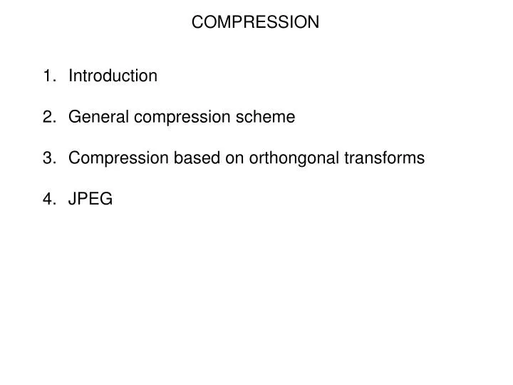
COMPRESSION. Introduction General compression scheme Compression based on orthongonal transforms JPEG. INTRODUCTION. Why to compress images ? digital images are nowadays ubiquitous : Science : remote sensing, medicine (CT, MRI, US ...) Industry : Machine vision

E N D
COMPRESSION • Introduction • General compression scheme • Compression based on orthongonal transforms • JPEG
INTRODUCTION • Why to compress images ? • digital images are nowadays ubiquitous : • Science : remote sensing, medicine (CT, MRI, US ...) • Industry : Machine vision • Web and electronic publishing, fax machines • Digital photography, video, TV • ... • infeasible to store or transmit without compression
INTRODUCTION 512 512 8 bpp = 262 KB 1 min. 38 s. at 28.8 Kb/s 512 512 3 channels 8 bpp = 768 KB 3.5 min. Photographic negative 35 mm scanned at 300 dpi, 3 channels = 18 MB 1 hour 20 min.
INTRODUCTION Digital photography of consumer camera 2592 1944 3 channels 8 bpc = 15 MB Digital radiography 34 43 cm at 70 m 12 bpp = 360 MB Satellite image 6000 4000 6 Channels 8 bpc = 1.4 GB
INTRODUCTION 512 512 200 planes 16 bpp = 100 MB . . . . . . . .
Spatial redundancy : Neighbour pixels have similar grey level (except in contours, textures, noise) because of their large low frequency content. INTRODUCTION Why compression is possible ?
INTRODUCTION Spatial redundancy : besides x, y also in z dimension
INTRODUCTION Spectral redundancy : channels are somehow related, they show mostly the same structures
INTRODUCTION Temporal redundancy : in video sequences time close frames are very similar. If camera is static, the background does not change.
INTRODUCTION • Types of compression • lossless / lossy (reversible / irreversible) • depending on the techinques (many) • How is the amount of compression measured ? • factor 5, 1:5, 1.6 bits/pixel (assuming 8bpp originally) • How to measure the image quality in lossy compression ? Depends on dynamic range S is the maximum pixel value Meaningless between different images
INTRODUCTION MSE or PSNR are quantitative measures. Measures related to subjective perceptual quality are more desirable
SCHEME How to achive compression ? A simple idea : use coding algorithms (e.g. Huffman, Lempel-Ziv) to assign short binary codes to frequent gray levels. 0 8 bits/pixel
SCHEME Could we previously transform the image so as to achieve a lower mean code length ?
SCHEME • How to achive compression ? • Steps of any compression scheme • Change of representation • Quantization of the new representation • Coding
SCHEME 1. Change of representation (reversible) histogram 255 -255 0 Are we compressing ? How many bits/bytes are needed to store the difference image ?
SCHEME 2. Quantization Reduce the number of possible differences to represent from 511 to, say, 16 but trying to keep the error low. [-255, -128] [-127, -32] [-31, -16] [-15, -4] -3 -2 -1 0 1 2 ...
SCHEME [-255, -128] [-127, -32] [-31, -16] [-15, -4] -3 -2 -1 0 1 2 ... -1 0 1 2 ... -192 -80 -24 -9 -3 -2 15 codes
SCHEME 3. Coding Mean length of a code Entropy : lower bound for L Huffman coding
a-2,-1 a-1,-1 a0,-1 a-2,0 a-1,0 SCHEME Actually, this example is kown as DPCM (differential or delta pulse code modulation) coding. Is the simplest case of predictive compression techiques : quantize and code the error of prediction of each pixel value from a neighbourhood of preceeding ones). Prediction is a fixed linear combination
ORTHOGONAL TRANSFORMS • The change of representation consist of : • Images are partitioned into non-overlapping blocks • Each block is seen as a matrix (i.e. element of a vectorial space) • Perform a fixed change of base • Many coefficients of the new representation can then • be removed • without perceptual difference • with a low MSE or high PSNR
x1i x2i i=1...N2/2 ORTHOGONAL TRANSFORMS An illustrative example : 1 2 blocks = 2d vectors N N
ORTHOGONAL TRANSFORMS The mean and variance of each coefficient is A first and weird change of representation : replace each x2i by the mean of x2 1:2 compression at least What is then the MSE ?
And how large is it ? Redundancy : most x1i x2i 2d histogram 255 255 x2 x2 0 0 255 255 0 0 x1 x1 ORTHOGONAL TRANSFORMS
x2 2d histogram y1 y2 x1 ORTHOGONAL TRANSFORMS Idea : a simple invertible coordinate transform can reduce and therefore the MSE
ORTHOGONAL TRANSFORMS Each block can be seen as an element of a 2d vectorial space in the canonical base : Rotation is a linear transform by an orthonormal matrix :
ORTHOGONAL TRANSFORMS • rows and columns of A are unitary and orthogonal • since they are rotations, orthonormal transforms do not change vectors norm neither total variance only that now
since they are rotations, orthonormal transforms do not change vectors norm neither total variance
ORTHOGONAL TRANSFORMS • rows of A are the vectors of the new base • the new coordinates of a vector are its projection = scalar product on to each base vector x2 y1 y2 x1
ORTHOGONAL TRANSFORMS This idea can be extended from 2d vectors to N N matrices: N=8 canonical base : N2 matrices N N • They form also a vectorial space
ORTHOGONAL TRANSFORMS • Can be changed to another othonormal base • These bases are formed by N2 orthonornal NN matrices Bij i, j = 1 ... N. matrix scalar product or projection orthonormal base if spans the N N matrix space and if else
ORTHOGONAL TRANSFORMS • Coefficients in the new base can be computed by block projection onto each base matrix Is a kind of simmilarity measure between F and Bkl • Of course, the new representation is a linear combination of base matrices
ORTHOGONAL TRANSFORMS • Which base ? Desirable properties of base for compression: • achieves good variance compactation : a few coefficients akl concetrate most of the total variance • A fast algorithm exists • Is independent of the image
ORTHOGONAL TRANSFORMS Discrete cosine transform (DCT) with if otherwise akl are the former coefficients
8 8 ORTHOGONAL TRANSFORMS Matrices of the 8 8 orthogonal base for DCT : u 0 1 2 3 4 5 6 7 0 1 2 3 4 5 6 v 7
ORTHOGONAL TRANSFORMS Variance compactation power of DCT : Matlab “dctdemo”
JPEG • JPEG = Joint Photographic Experts Group, sponsored by ISO and CCIT to develop a compression standard for still images. • Three parts : • Base system : simple and efficient algorithm for most images, based on DCT • A lossless compression scheme (predictive + Huffman) • Extensions (12 bits images, hierarchical)
JPEG Encoding : In general a color image Controls image quality and compression factor Decoding : reverse the order
JPEG 8 8 blocks
JPEG 1. Change of representation DCT, integer arithmetic
JPEG 2. Non-uniform quantization : a possibly different step for each coefficient Nearest neighbour Sample quatization Matrix (steps)
. . . . . . JPEG 1260/16=78.75
JPEG 3. Coding • DPCM on G(0,0) • Run-length on other G(i,j) : zig-zag transversal + keep • skip and value, where skip is the number of zeros and value is the next non-zero component • Huffmann coding of all these values
JPEG Error :
JPEG original DCT coefficients Y I Q quantized coefficients compressed http://www.cs.sfu.ca/CC/365/li/interactive-jpeg/Ijpeg.html