Download
1 / 42
440 likes | 479 Views
Temporal Databases. Outline. Spatial Databases Indexing, Query processing Temporal Databases Spatio-temporal …. Temporal DBs – Motivation. Conventional databases represent the state of an enterprise at a single moment of time Many applications need information about the past

E N D
Outline • Spatial Databases • Indexing, Query processing • Temporal Databases • Spatio-temporal • ….
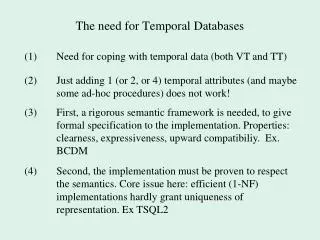
Temporal DBs – Motivation • Conventional databases represent the state of an enterprise at a single moment of time • Many applications need information about the past • Financial (payroll) • Medical (patient history) • Government • Temporal DBs: a system that manages time varying data
Comparison • Conventional DBs: • Evolve through transactions from one state to the next • Changes are viewed as modifications to the state • No information about the past • Snapshot of the enterprise • Temporal DBs: • Maintain historical information • Changes are viewed as additions to the information stored in the database • Incorporate notion of time in the system • Efficient access to past states
Temporal Databases • Temporal Data Models: extension of relational model by adding temporal attributes to each relation • Temporal Query Languages: TQUEL, SQL3 • Temporal Indexing Methods and Query Processing
Taxonomy of time • Transaction time databases • Transaction time is the time when a fact is stored in the database • Valid time databases: • Valid time is the time that a fact becomes effective in reality • Bi-temporal databases: • Support both notions of time
Example • Sales example: data about sales are stored at the end of the day • Transaction time is different than valid time • Valid time can refer to the future also! • Credit card: 03/13-04/16
Transaction Time DBs • Time evolves discretely, usually is associated with the transaction number: • A record R is extended with an interval [t.start, t.end). When we insert an object at t1 the temporal attributes are updated -> [t1, now) • Updates can be made only to the current state! • Past cannot be changed • “Rollback” characteristics T1 -> T2 -> T3 -> T4 ….
Transaction Time DBs • Deletion is logical (never physical deletions!) • When an object is deleted at t2, its temporal attribute changes from [t1, now) [t1, t.t2) (lifetime) • Object is “alive” from insertion to deletion time, ex. t1 to t2. If “now” then the object is still alive time
Transaction Time DBs id Database evolves through insertions and deletions
Transaction Time DBs • Requirements for index methods: • Store past logical states • Support addition/deletion/modification changes on the objects of the current state • Efficiently access and query any database state
Transaction Time DBs • Queries: • Timestamp (timeslice) queries: ex. “Give me all employees at 05/94” • Range-timeslice: “Find all employees with id between 100 and 200 that worked in the company on 05/94” • Interval (period) queries: “Find all employees with id in [100,200] from 05/14 to 06/16”
Valid Time DBs • Time evolves continuously • Each object is a line segment representing its time span (eg. Credit card valid time) • Support full operations on interval data: • Deletion at any time • Insertion at any time • Value change (modification) at any time (no ordering)
Valid Time DBs • Deletion is physical: • No way to know about the previous states of intervals • The notion of “future”, “present” and “past” is relative to a certain timestamp t
Valid Time DBs The reality “best know now !”
Valid Time DBs • Requirements for an Index method: • Store the latest collection of interval-objects • Support add/del/mod changes to this collection • Efficiently query the intervals in the collection • Timestamp query • Interval (period) query
Bitemporal DBs • A transaction-time Database, but each record is an interval (plus the other attributes of the record) • Keeping the evolution of a dynamic collection of interval-objects • At each timestamp, it is a valid time database
Bitemporal DBs • Requirements for access methods: • Store past/logical states of collections of objects • Support add/del/mod of interval objects of the current logical state • Efficient query answering
Temporal Indexing • Straight-forward approaches: • B+-tree and R-tree • Problems? • Transaction time: • Snapshot Index, TSB-tree, MVB-tree, MVAS • Valid time: • Interval structures: Segment tree, even R-tree • Bitemporal: • Bitemporal R-tree
Temporal Indexing • Lower bound on answering timeslice and range-timeslace queries: • Space O(n/B), search O(logBn + s/B) • n: number of changes, s: answer size, B page capacity Range-timeslice: “Find all employees with id between 100 and 200 that worked in the company on 05/94”
Transaction Time Environment • Assume that when an event occurs in the real world it is inserted in the DB • A timestamp is associated with each operation • Transaction timestamps are monotonically increasing • Previous transactions cannot be changed we cannot change the past
Example • Time evolving set of objects: employees of a company • Time is discrete and described by a succession of non-negative integers: 1,2,3, … • Each time instant changes may happen, i.e., addition, deletion or modification • We assume only insertion & deletion : modifications can be represented by a deletion and an insertion
Records • Each object is associated with: • An oid (key, time invariant, eid) • Attributes that can change (salary) • A lifespan interval [t.start, t.end) • An object is alive from the time it inserted in the set, until it was deleted • At insertion time deletion is unknown • Deletions are logical: we change the now variable to the current time, [t1, now) [t1, t2)
Evolving set • The state S(t) of the evolving set at t is defined as: “the collection of alive objects at t” • The number of changes n represents a good metric for the minimal space needed to store the evolution
Evolving sets • A new change updates the current state S(t) to create a new state t1 ti time t2 a a,f,g a,h S(ti)
Transaction-time Queries • Pure-timeslice • Range-timeslice • Pure-exact match
Snapshot Index • Snapshot Index, is a method that answers efficiently pure-timeslice queries • Based on a main memory method that solves the problem in O(a+log2n), O(n) space • External memory: O(a/B + logBn)
MM solution • Copy approach: O(a + logn) but O(n2) space • Log approach: O(n) space but O(n) query time • We should combine the fast query time with the small space (and update)
Assumptions • Assumptions (for clarity) • At each time instant there exist exactly one change • Each object is named by its creation time
Access Forest • A double linked list L. Each new object is appended at the right end of L • A deleted object is removed from L and becomes the next child of its left sibling in L • Each object stores a pointer to its parent object. Also a parent object points to its first and last children • So, each node has the following pointers: parent, prev, next, Pcs, Pce
AF example SP 29 70 46 1 60 64 15
Additional structures • A hashing scheme that keeps pointers to the positions of the alive elements in L • An array A that stores the time changes. For each time change instant, it keeps the pointer to the current last object in L
Properties of AF • In each tree of the AF the start times are sorted in preorder fashion • The lifetime of an object includes the lifetimes of its descendants • The intervals of two consecutive children under the same parent may have the following orderings: si < ei < si+1 <ei+1 or si< si+1<ei < ei+1
Searching • Find all objects alive at tq • Use A to find the starting object in the access forest L (O(logn)) • Traverse the access forest and report all alive objects at tq O(a) using the properties
Searching in AF • Given query time q: • Use table A to find the time of the last object in L at time q. Say node Y. • Starting from Y go up (if it has a parent) recursively • For each node in the path from Y to the current node in list L (or Y itself if it is right now in L) • Recursively go to the left sibling • Visit the rightmost child
Disk based Solution • Keep changes in pages as it was a Log • Use hashing scheme to find objects by name (update O(1)) • Acceptor : the current page that receives objects
Definitions • A page is useful for the following time instants: • I-useful: while this page was the acceptor block • II-useful: for all time instants for which it contains at least uB “alive” records • u is the usefulness parameter
Meta-evolution • From the actual evolution of objects, now we have the evolution of pages! meta-evolution • The “lifetime” of a page is its usefulness
Searching • Find all alive objects at tq Find all useful pages at tq • The search can be done in O(a/B + logBn)
Copying procedure • To maintain the answer in few pages we need clustering: controlled copying • If a page has less than uB alive objects, we artificially delete the remaining alive objects and copy them to the acceptor bock
Optimal Solution • We can prove that the SI is optimal for pure-timeslice queries: • O(n) space, O(a/B + logBn) query and O(1) update (expected, using hashing)