Multi-Level Logic Synthesis Slides courtesy of Andreas Kuehlmann (Cadence)

Multi-Level Logic Synthesis Slides courtesy of Andreas Kuehlmann (Cadence)

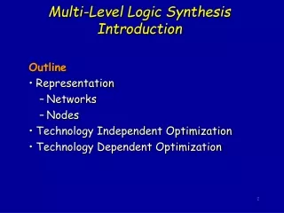
Finite State Machine Model M(X,Y,S,S0,d,l): X: Inputs Y: Outputs S: Current State S0: Initial State(s) d: X ´ S ® S (next state function) l: X ´ S ® Y (output function) Y=(y1,y2,…,yn) X=(x1,x2,…,xn) l S’=(s’1,s’2,…,s’n) S=(s1,s2,…,sn) d D • Delay element: • Clocked: synchronous • single-phase clock, multiple-phase clocks • Unclocked: asynchronous

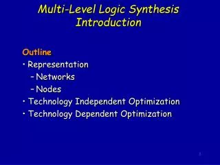
General Logic Structure • Combinational optimization • keep latches/registers at current positions, keep their function • optimize combinational logic in between • Sequential optimization • change latch position/function

Optimization Criteria for Synthesis The optimization criteria for multi-level logic is to minimizesome function of: • Area occupied by the logic gates and interconnect (approximated by literals = transistors in technology independent optimization) • Critical path delayof the longest path through the logic • Degree of testability of the circuit, measured in terms of the percentage of faults covered by a specified set of test vectors for an approximate fault model (e.g. single or multiple stuck-at faults) • Power consumed by the logic gates • Noise Immunity • Place-ability, Wire-ability while simultaneously satisfying upper or lower bound constraints placed on these physical quantities

Example: Area-Delay Trade-off

Two-Level (PLA) vs. Multi-Level E.g. Standard Cell Layout PLA control logic constrained layout highly automatic technology independent multi-valued logic input, output, state encoding Very predictable Multi-level Logic all logic general (e.g. standard cell, regular blocks,..) automatic partially technology independent some ideas part of multi-level logic Very hard to predict

General Approaches to Synthesis • PLA Synthesis: • theory well understood • predictable results in a top-down flow • Multi-Level Synthesis: • optimization criteria very complex • except niches, no general theory available • greedy optimization approach • incrementally improve along various dimensions of the criteria • attempt a change, accept if criteria improves, otherwise reject • works on common design representation (circuit or network representation)

Transformation-based Synthesis • all modern synthesis systems are built that way • set of transformations that change network representation • work on uniform network representation • “script” of “scenario” that can combine those transformations • transformations differ in: • the scope they are applied • local scope versus global restructuring • the domain they optimize • combinational versus sequential • timing versus area • technology independent versus technology dependent • the underlying algorithms they use • BDD based, SAT based, structure based

Network Representation Boolean network: • directed acyclic graph (DAG) • node logic function representation fj(x,y) • node variableyj: yj= fj(x,y) • edge (i,j)if fjdepends explicitly on yi Inputs x = (x1, x2,…,xn ) Outputs z = (z1, z2,…,zp ) External don’t cares d1(x), d2(x) ,…, dp(x)

Technology independent Optimizations Technology Dependent Optimizations RTL to Network Transformation Technology Mapping Test Preparation Typical Synthesis Scenario - read Verilog - control/data flow analysis - basic logic restructuring - crude measures for goals - use logic gates from target cell library - timing optimization - physically driven optimizations - improve testability - test logic insertion

Local versus Global Transformations • Local transformations optimize the function of one node of thenetwork • smaller area • faster performance • map to a particular set of cells • Global transformations restructure the entire network • merging nodes • splitting nodes • removing/changing connections between nodes • Node representation: • SOP, POS • BDD • Factored forms • keep size bounded to avoid blow-up of local transformations

Sum of Products (SOP) Example: abc’+a’bd+b’d’+b’e’f (sum of cubes) Advantages: • easy to manipulate and minimize • many algorithms available (e.g. AND, OR, TAUTOLOGY) • two-level theory applies Disadvantages: • Not representative of logic complexity. For example f=ad+ae+bd+be+cd+ce f’=a’b’c’+d’e’ These differ in their implementation by an inverter. • hence not easy to estimate logic; difficult to estimate progress during logic manipulation

Reduced Ordered BDDs • like factored form, represents both function and complement • like network of muxes, but restricted since controlled by primary input variables • not really a good estimator for implementation complexity

Factored Forms Example:(ad+b’c)(c+d’(e+ac’))+(d+e)fg Advantages • good representative of logic complexity f=ad+ae+bd+be+cd+ce f’=a’b’c’+d’e’  f=(a+b+c)(d+e) • in many designs (e.g. complex gate CMOS) the implementation of a function corresponds directly to its factored form • good estimator of logic implementation complexity • doesn’t blow up easily Disadvantages • not as many algorithms available for manipulation • hence often just convert into SOP before manipulation

Factored Forms Note: literal count »transistor count » area • however, area also depends on • wiring • gate size etc. • therefore very crude measure

Factored Forms When measured in terms of number of inputs, there are functions whose size is exponential in sum of products representation, but polynomial in factored form. Example: Achilles’ heel function There are n literals in the factored form and (n/2)2n/2 literals in the SOP form. Factored forms are useful in estimating area and delay in a multi-level synthesis and optimization system. In many design styles (e.g. complex gate CMOS design) the implementation of a function corresponds directly to its factored form.

Factored Forms Factored forms cam be graphically represented as labeled trees, called factoring trees, in which each internal node including the root is labeled with either +or, and each leaf has a label of either a variable or its complement. Example:factoring tree of ((a’+b)cd+e)(a+b’)+e’

Factored Forms The size of a factored form F (denoted (F )) is the number of literals in the factored form. Example:(( a+b)ca’) = 4((a+b+cd)(a’+b’)) = 6 A factored form is optimal if no other factored form (for that function) has fewer literals.

SOPs forms are used as the internal representation of logic functions in most multi-level logic optimization systems. Advantages good algorithms for manipulating them are available Disadvantages performance is unpredictable - they may accidentally generate a function whose SOP form is too large factoring algorithms have to be used constantly to provide an estimate for the size of the Boolean network, and the time spent on factoring may become significant Possible solution avoid SOP representation by using factored forms as the internal representation this is not practical unless we know how to perform logic operations directly on factored forms without converting to SOP forms extensions to factored forms of the most common logic operations have been partially provided Factored Forms

Manipulation of Boolean Networks Basic Techniques: • structural operations (change topology) • algebraic • Boolean • node simplification (change node functions) • don’t cares • node minimization

Structural Operations Restructuring Problem:Given initial network, find best network. Example:f1 = abcd+abce+ab’cd’+ab’c’d’+a’c+cdf+abc’d’e’+ab’c’df’ f2 = bdg+b’dfg+b’d’g+bd’eg minimizing, f1 = bcd+bce+b’d’+a’c+cdf+abc’d’e’+ab’c’df’ f2 = bdg+dfg+b’d’g+d’eg factoring, f1 = c(b(d+e)+b’(d’+f)+a’)+ac’(bd’e’+b’df’) f2 = g(d(b+f)+d’(b’+e)) decompose, f1 = c(x+a’)+ac’x’ f2 = gx x = d(b+f)+d’(b’+e) Two problems: • find good common subfunctions • effect the division

Structural Operations Basic Operations: 1. Decomposition (single function) f = abc+abd+a’c’d’+b’c’d’  f = xy+x’y’ x = ab y = c+d 2. Extraction (multiple functions) f = (az+bz’)cd+e g = (az+bz’)e’ h = cde  f = xy+e g = xe’ h = ye x = az+bz’ y = cd 3. Factoring (series-parallel decomposition) f = ac+ad+bc+bd+e  f = (a+b)(c+d)+e

Structural Operations 4. Substitution g = a+b f = a+bc  f = g(a+c) 5. Collapsing (also called elimination) f = ga+g’b g = c+d  f = ac+ad+bc’d’ g = c+d Note:“division” plays a key role in all of these

Factoring vs. Decomposition Factoringf=(e+g’)(d(a+c)+a’b’c’)+b(a+c) Decomposition:y(b+dx)+xb’y’ Note: this is similar to BDD collapsing of common nodes and using negative pointers. But not canonical, so don’t have perfect identification of common nodes. Tree DAG

Value of a Node and Elimination where ni = number of times literalsyjand yj’ occur in factored form fi lj = number of literals in factored fj with factoring without factoring value = (without factoring) - (with factoring) Can treat yj and yj’ the same since ( Fj ) = ( Fj’ ).

Value of a Node and Elimination Literals before = 5+7+5 = 17 Literals after = 9+15 = 24 --- 7 x Difference after - before = value = 7 But we may not have the same value if we were to eliminate, simplify and then re-factor.

Value of a Node and Elimination value=3 Note: value of a node can change during elimination

Why Use Algebraic Methods? • need spectrum of operations • algebraic methods provide fast algorithms • treat logic function like a polynomial • efficient data structures • fast methods for manipulation of polynomials available • loss of optimality, but results quite good • can iterate and interleave with Boolean operations • in specific instances slight extensions available to include Boolean methods

Weak Division Weak division is a specific example of algebraic division. DEFINITION: Given two algebraic expressions F and G, a division is called weak division if • it is algebraic and • R has as few cubes as possible. The quotient H resulting from weak division is denoted by F/G. THEOREM: Given expressions F and G, H and R generated by weak division are unique.

Division - What do we divide with? • Weak_Div provides a methods to divide an expression for a given divisor • How do we find a “good” divisor? • Restrict to algebraic divisors • generalize to Boolean divisors • Problem: • Given a set of functions { Fi }, find common weak (algebraic) divisors.

Application - Decomposition • Decomposition is the same as factoring except: • divisors are added as new nodes in the network. • the new nodes may fan out elsewhere in the network in both positive and negative phases Algorithm DECOMP(fi) { k = CHOOSE_KERNEL(fi) if (k == 0) return fm+j = k // create new node m + j fi = (fi/k)ym+j+(fi/k’)y’m+j+r // change node i using new // node for kernel DECOMP(fi) DECOMP(fm+j) } Similar to factoring, we can define QUICK_DECOMP: pick a level 0 kernel and improve it. GOOD_DECOMP: pick the best kernel.

Re-substitution • Idea: An existing node in a network may be a useful divisor in another node. If so, no loss in using it (unless delay is a factor). • Algebraic substitution consists of the process of algebraically dividing the function fi at node i in the network by the function fj (or by f’j) at node j. During substitution, if fj is an algebraic divisor of fj, then fi is transformed into fi = qyj + r (or fi = q1yj + q0y’j + r ) • In practice, this is tried for each node pair of the network. n nodes in the network  O(n2) divisions. fi yj fj

Extraction • Recall: Extraction operation identifies common sub-expressions and manipulates the Boolean network. • Combine decomposition and substitution to provide an effective extraction algorithm. Algorithm EXTRACT foreach node n {DECOMP(n) // decompose all network nodes } foreach node n { RESUB(n) // resubstitute using existing nodes } ELIMINATE_NODES_WITH_SMALL_VALUE }

Extraction Kernel Extraction:1. Find all kernels of all functions2. Choose kernel intersection with best “value”3. Create new node with this as function4. Algebraically substitute new node everywhere5. Repeat 1,2,3,4 until best value  threshold New Node

Multi-Level Logic Synthesis Slides courtesy of Andreas Kuehlmann (Cadence)