Download
1 / 69
690 likes | 788 Views
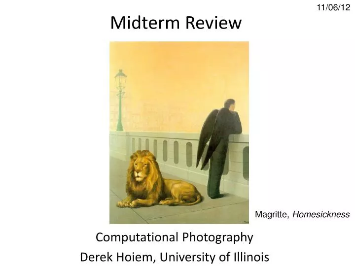
11/06/12. Midterm Review. Computational Photography Derek Hoiem, University of Illinois. Magritte, Homesickness. Major Topics. Linear Filtering How it works Template and Frequency interpretations Image pyramids and their applications

E N D
11/06/12 Midterm Review Computational Photography Derek Hoiem, University of Illinois Magritte, Homesickness
Major Topics • Linear Filtering • How it works • Template and Frequency interpretations • Image pyramids and their applications • Sampling (Nyquist theorem, application of low-pass filtering) • Light and color • Lambertian shading, shadows, specularities • Color spaces (RGB, HSV, LAB) • Techniques • Finding boundaries: intelligent scissors, graph cuts, where to cut and why • Texture synthesis: idea of sampling patches to synthesize, filling order • Compositing and blending: alpha compositing, Laplacian blending, Poisson editing • Warping • Transformation matrices, homogeneous coordinates, solving for parameters via system of linear equations • Modeling shape • Averaging and interpolating sets of points • Compressing and finding dominant modes of variation using PCA
Major Topics • Camera models and Geometry • Pinhole model: diagram, intrinsic/extrinsic matrices, camera center (or center of projection), image plane • Focal length, depth of field, field of view, aperture size • Vanishing points and vanishing lines (what they are, how to find them) • Measuring relative lengths based on vanishing points and horizon • Interest points • Trade-offs between repeatability and distinctiveness for detectors and descriptors • Harris (corner) detectors and Difference of Gaussian (blob) detectors • SIFT representation: what transformations is it robust to or not robust to • Image stitching • Solving for homography • RANSAC for robust detection of inliers • Object recognition and search • Use of “visual words” to speed search • Idea of geometric verification to check that points have consistent geometry
Studying for Midterm • Roughly 80% is related to topics in bold (linear filtering, warping, camera models and geometry) • No book, no notes, no computers/calculators allowed • Bring a pencil or pen
Today’s review • Light • Camera capture and geometry • Image filtering • Region selection and compositing • Solving for transformations Purposes • Remind you of key concepts • Chance for you to ask questions
1. Light and color • Lighting • Lambertian shading, shadows, specularities • Color spaces (RGB, HSV, LAB)
How is light reflected from a surface? Depends on • Illumination properties: wavelength, orientation, intensity • Surface properties: material, surface orientation, roughness, etc. light source λ ?
Lambertian surface • Some light is absorbed (function of albedo) • Remaining light is reflected equally in all directions (diffuse reflection) • Examples: soft cloth, concrete, matte paints light source light source λ λ diffuse reflection absorption
Diffuse reflection Intensity does depend on illumination angle because less light comes in at oblique angles. albedo directional source surface normal image intensity Slide: Forsyth
1 2
Diffuse reflection Perceived intensity does not depend on viewer angle. • Amount of reflected light proportional to cos(theta) • Visible solid angle also proportional to cos(theta) http://en.wikipedia.org/wiki/Lambert%27s_cosine_law
Specular Reflection • Reflected direction depends on light orientation and surface normal • E.g., mirrors are fully specular Flickr, by suzysputnik light source λ specular reflection Flickr, by piratejohnny
Many surfaces have both specular and diffuse components • Specularity= spot where specular reflection dominates (typically reflects light source) Photo: northcountryhardwoodfloors.com
Questions 09/08/11 1. Possible factors: albedo, shadows, texture, specularities, curvature, lighting direction
Pinhole Camera . Optical Center (u0, v0) . . f Z Y v . Camera Center (tx, ty, tz) u Useful figure to remember
Projection Matrix R jw t kw Ow iw
Single-view metrology 5 4 3 2 1
Adding a lens “circle of confusion” • A lens focuses light onto the film • There is a specific distance at which objects are “in focus” • other points project to a “circle of confusion” in the image • Changing the shape of the lens changes this distance
Focal length, aperture, depth of field A lens focuses parallel rays onto a single focal point • focal point at a distance f beyond the plane of the lens • Aperture of diameter D restricts the range of rays F focal point optical center (Center Of Projection) Slide source: Seitz
The aperture and depth of field Slide source: Seitz Two ways to increase depth of field: • Decrease aperture size • Increase focus distance (zoom) F-number (f/#) =focal_length / aperture_diameter - E.g., f/16 means that the focal length is 16 times the diameter - When you set the f-number of a camera, you are setting the aperture f / 5.6 f / 32 Flower images from Wikipedia http://en.wikipedia.org/wiki/Depth_of_field
The Photographer’s Great Compromise What we want More spatial resolution Broader field of view More depth of field More temporal resolution More light How we get it Cost Increase focal length Light, FOV Decrease focal length DOF Decrease aperture Light Increase aperture DOF Shorten exposure Light Lengthen exposure Temporal Res
Discretization • Because pixel grid is discrete, pixel intensities are determined by a range of scene points
Color Sensing: Bayer Grid • Estimate RGB at each cell from neighboring values http://en.wikipedia.org/wiki/Bayer_filter Slide by Steve Seitz
Color spaces RGB LAB 0,1,0 Y=0 Y=0.5 Y=1 Cr Cb HSV 1,0,0 YCbCr 0,0,1
Contrast enhancement / balancing • Gamma correction • Histogram equalization Cumulative Histograms
3. Linear filtering • Can think of filtering as • A function in the spatial domain (e.g., compute average of each 3x3 window) • Template matching • Modifying the frequency of the image
Filtering in spatial domain 1 1 1 1 1 1 1 1 1 • Slide filter over image and take dot product at each position ?
Filtering in spatial domain 1 0 -1 2 0 -2 1 0 -1 * =
Filtering in frequency domain • Can be faster than filtering in spatial domain (for large filters) • Can help understand effect of filter • Algorithm: • Convert image and filter to fft (fft2 in matlab) • Pointwise-multiply ffts • Convert result to spatial domain with ifft2
Filtering in frequency domain FFT FFT = Inverse FFT
Filtering in frequency domain • Linear filters for basic processing • Edge filter (high-pass) • Gaussian filter (low-pass) [-1 1] Gaussian FFT of Gradient Filter FFT of Gaussian
Filtering Why does the Gaussian give a nice smooth image, but the square filter give edgy artifacts? Gaussian Box filter
Question • Use filtering to find pixels that have at least three white pixels in among the 8 surrounding pixels • Write down a filter that will compute the gradient in the y-direction: gradx(y,x) = im(y+1,x)-im(y,x) for each x, y
Question Filtering Operator a) _ = D * B b) A = _ * _ c) F = D * _ d) _ = D * C 3. Fill in the blanks: A B E G C F D H I
Question • Match the spatial domain image to the Fourier magnitude image 2 3 1 4 5 B C E A D
Matching with filters • Goal: find in image • Method 2: SSD True detections Thresholded Image 1- sqrt(SSD) Input
Matching with filters • Goal: find in image • Method 3: Normalized cross-correlation mean template mean image patch Matlab: normxcorr2(template, im)
Matching with filters • Goal: find in image • Method 3: Normalized cross-correlation True detections Thresholded Image Input Normalized X-Correlation
Subsampling by a factor of 2 Problem: This approach causes “aliasing” • Throw away every other row and column to create a 1/2 size image
Nyquist-Shannon Sampling Theorem • When sampling a signal at discrete intervals, the sampling frequency must be 2 fmax • fmax = max frequency of the input signal • This will allows to reconstruct the original perfectly from the sampled version good v v v bad
Algorithm for downsampling by factor of 2 • Start with image(h, w) • Apply low-pass filter • im_blur = imfilter(image, fspecial(‘gaussian’, 7, 1)) • Sample every other pixel • im_small = im_blur(1:2:end, 1:2:end);
Subsampling without pre-filtering 1/2 1/4 (2x zoom) 1/8 (4x zoom) Slide by Steve Seitz
Subsampling with Gaussian pre-filtering Gaussian 1/2 G 1/4 G 1/8 Slide by Steve Seitz
Sampling Why does a lower resolution image still make sense to us? What do we lose? Image: http://www.flickr.com/photos/igorms/136916757/
Gaussian pyramid • Useful for coarse-to-fine matching • Applications include multi-scale object detection, image alignment, optical flow, point tracking
Computing Gaussian/Laplacian Pyramid Gaussian Pyramid 2-level Laplacian Pyramid Useful figure to remember http://sepwww.stanford.edu/~morgan/texturematch/paper_html/node3.html