Download
1 / 21
210 likes | 357 Views
Alternative routes to the 1D discrete nonpolynomial Schrödinger equation. Boris Malomed Dept. of Physical Electronics, Faculty of Engineering, Tel Aviv University, Tel Aviv, Israel Goran Gligorić and Ljupco Hadžievski Vinća Institute of Nuclear Sciences, Belgrade, Serbia Aleksandra Maluckov

E N D
Alternative routes to the 1D discrete nonpolynomial Schrödinger equation Boris Malomed Dept. of Physical Electronics, Faculty of Engineering, Tel Aviv University, Tel Aviv, Israel Goran Gligorić and Ljupco Hadžievski Vinća Institute of Nuclear Sciences, Belgrade, Serbia Aleksandra Maluckov Faculty of Sciences and Mathematics, University of Niš, Niš, Serbia Luca Salasnich Department of Physics “Galileo Galilei” Universitá di Padova, Padua, Italy
The topic of the work: approximation of the Gross-Pitaevskii equation for BEC by means of discrete models, in the presence of a deep optical lattice. We report derivation of a new model, and its comparison with the previously know one. A simulating discussion with Dmitry Pelinovsky is appreciated. Some revious works on the topic of the discrete approximation for BEC: A. Trombettoni and A. Smerzi, Phys. Rev. Lett. 86, 2353 (2001); F.Kh. Abdullaev, B. B. Baizakov, S.A. Darmanyan, V.V. Konotop & M. Salerno, Phys. Rev. A 64, 043606 (2001); G.L. Alfimov, P. G. Kevrekidis, V.V. Konotop & M. Salerno, Phys. Rev. E 66, 046608 (2002); R. Carretero-González & K. Promislow, Phys. Rev. A 66, 033610 (2002); N.K. Efremidis & D.N. Christodoulides, ibid. 67, 063608 (2003); M. A. Porter, R. Carretero-González, P. G. Kevrekidis & B. A. Malomed, Chaos 15, 015115 (2005); G. Gligorić, A. Maluckov, Lj. Hadžievski & B.A. Malomed, ibid. 78, 063615 (2008).
The starting point: the rescaled three-dimensional (3D)Gross-Pitaevskii equation (GPE) for the normalized mean-field wave function. The GPE includes the transverse parabolic trapping potential and the longitudinal (axial) optical-lattice (OL) periodic potential:
The first (“traditional”) way of the derivation of the 1D discrete model: start by reducing the dimension of the continual equationfrom 3 to 1, and thendiscretize the effective 1D equation.
The discretization of the one-dimensional NPSE leads to the DNPSE [A. Maluckov, Lj. Hadžievski, B. A. Malomed, and L. Salasnich, Phys. Rev. A 78, 013616 (2008)], through the expansion over a set of localized wave functions
The new (“second”) route to the derivation of the 1D discrete model: first perform the discretization of the underlying 3D GPE in the direction of z, and then perform the reduction of the dimension. The two operations are expected to be non-communitative.
The reduction of the semi-discrete equation to the 1Ddiscrete form.
At the first glance, this system seems very complex, and completely different from the DNPSE equation for the discrete wave function, fn(t), which was derived by means of the “traditional approach”. Our objective is to find and comparefamilies of fundamental discrete solitons in both models, the “traditional simple”, and “new complex” ones.
The distinction between the “traditional” and “new” models is also seen in the difference between their Hamiltonians, while they share the same expression for the norm (P):
First, we consider the modulational instability of CW (uniform) waves, fn(t) = U exp(-iμt),in the case of the attractive nonlinearity, g < 0. The CW solutions are unstablein regions below the respective curves (q is the wavenumber of the modulational perturbations):
Comparison of the shapes of unstaggered onsite-centered discrete solitons: transverse widths (σn) at the central site of the soliton, and two sites adjacent to the center, in the two models, for C = 0.2 and C = 0.8. Chains of symbols: the “old” model; curves: the “new” one.
The same comparison for unstaggered intersite-centered solitons:
Stationary soliton solutions with chemical potentialμare looked for as fn = Fn exp(-iμt), with real Fn, for two soliton families: onsite-centered and intersite-centered ones. Then, the families may be described by dependences of the norm vs. the chemical potential,
The comparison of the P(μ) characteristics for the family of onsite-centered solitons, at C = 0.2 and C = 0.8. Note that the VK stability criterion, dP/dμ < 0, generally, does not apply to the model with the nonpolynomial nonlinearity.
The same comparison for families of intersite-centered solitons, also for C = 0.2 and C = 0.8:
A similar comparison of values of the free energy for both models, G = H – μP, again for C = 0.2 and C = 0.8. Left and right curves in both panels pertain to on-site and inter-site solitons, respectively:
The comparison of dynamical properties of the discrete solitons in both models. In particular, realeigenvalues (“ev”), accounting for the instability of a part of the family of the onsite-centeredsolitons (a) and of the intersite-centered soliton family (b), at C = 0.8, as functions of μ, have the following form in both models (the intersite solitons are completely unstable in both models; onsite solitons have their stability region):
CONCLUSIONS There are two alternative ways to derive the 1D discrete equation for BEC trapped in the combination of the tight transverse confining potential and deep axial optical lattice: (1) First, reduce the dimension from 3 to 1, arriving at the nonpolynomial NLS equation, and then subject it to the discretization; or (2) First, apply the discretization to the 3D equation, reducing it to a semi-discrete form, and then eliminate (by averaging) the two transverse dimensions.
Because the reduction of the dimension and the discretizationdo not commute, these alternative routes of the derivation lead to two models which seem completely different: the earlier known discrete nonpolynomial NLS equation (obtained by means of the former method), or the model obtained by means of the latter method, which, apparently, has a much more complexform.
However, despite the very different form of the two models, they produce nearly identical results for the shape of unstaggered discrete solitons of both the onsite- and intersite-centered types, and virtually identical conclusions about their stability. Additional numerical analysis demonstrates that the character of the collapse in both discrete models is also essentially the same (note that both models are capable to predict the collapse in the framework of the 1Ddiscrete approximation), as well as regions of the mobility of the solitons.
The general conclusion: The approximation of the dynamical behavior of the 3D condensate in the present setting by the 1D discrete model is reliable, as two very different models yield almost identical eventual results.