Download
1 / 24
250 likes | 273 Views
Spatial Data Analysis. Interpolation of Surfaces. Spatial Interpolation. Spatial interpolation is the prediction of exact values of attributes at un-sampled locations from measurements made at control points within the same area. z?. z?. z?. z?. z?. z?. z?. Spatial Interpolation.

E N D
Spatial Data Analysis Interpolation of Surfaces
Spatial Interpolation Spatial interpolation is the prediction of exact values of attributes at un-sampled locations from measurements made at control points within the same area. z? z? z? z? z? z? z?
Spatial Interpolation Automating interpolation is performed with GIS: Proximity Polygons Inverse Distance Weighted Spatial Average Spline Smoothing Krigging
Interpolation of Surfaces Inverse Distance Weighted
Spatial Interpolation Proximity Polygons This technique was introduced a century ago by Thiessen (1911) Abrupt change at edges is the main pitfall of this method
Inverse Distance Weighted Spatial Average Inverse distance weighting models work on the premise that observations further away should have their contributions diminished according to how far away they are. The simplest model involves calculating the weighted mean for all of the observations
Inverse Distance Weighted Spatial Average While the weight is the inverse of the distance it is from the target point raised to a power α By defining the higher {power} option, more emphasis can be put on the nearest points. Thus, nearby data will have the most influence, and the surface will have more detail (be less smooth). As the power increases, the interpolated values begin to approach the value of the nearest sample point. Specifying a lower value for power will provide a bit more influence to surrounding points a little farther away.
Inverse Distance Weighted Spatial Average Effect of α: Source Data
Inverse Distance Weighted Spatial Average Effect of α: α = 1
Inverse Distance Weighted Spatial Average Effect of α: α = 3
Inverse Distance Weighted Spatial Average Many GIS packages provide this kind of inverse distance model for interpolation, as it is simple to implement and to understand. Often the model is generalised in a number of ways: a faster rate of distance decay may be provided, by including a power function of distance, α >1, rather than simple linear distance. While any α value convenient for a given application may be used, common practice is to use distance (α = 1) or distance squared (α = 2).
Interpolation of Surfaces Spline Interpolation
Spline Interpolation Method Definition: The Spline method is an interpolation method that estimates values using a mathematical function that minimizes overall surface curvature, resulting in a smooth surface that passes exactly through the input points.
Spline Interpolation Method • The basic form of the minimum curvature Spline interpolation imposes the following two conditions on the interpolant: • The surface must pass exactly through the data points. • The surface must have minimum curvature—the cumulative sum of the squares of the second derivative terms of the surface taken over each point on the surface must be a minimum.
Spline Interpolation Method Spline bends a sheet of rubber that passes through the input points while minimizing the total curvature of the surface. It fits a mathematical function to a specified number of nearest input points while passing through the sample points. This method is best for generating gently varying surfaces such as elevation, water table heights, or pollution concentrations.
Spline Interpolation Method There are two Spline methods: Regularized and Tension. The Regularized method creates a smooth, gradually changing surface with values that may lie outside the sample data range. The Tension method controls the stiffness of the surface according to the character of the modeled phenomenon. It creates a less smooth surface with values more closely constrained by the sample data range.
Interpolation of Surfaces Krigging
Krigging Krigging is a statistical interpolation method that is optimal in the sense that it makes best use of what can be inferred about the spatial structure in the surface to be interpolated from an analysis of control point data. In IDW we calculate the weights from the inverse of distance raised to some power. Krigging finds the optimum weights for the data values in the interpolation at each unknown location.
Krigging • To interpolate in this way, three distinct steps are involved: • Producing a description of the spatial vario-gram in the sample control data. • Summarizing this spatial variation by a regular mathematical function • Using this model to determine the interpolation weights