Download
1 / 54
540 likes | 563 Views
Distributed Transaction Management – 2003. Jyrki Nummenmaa http://www.cs.uta.fi/~dtm jyrki@cs.uta.fi. Physical clock synchronisation. Coordinated universal time. Atomic clocks based on atomic oscillations are the most accurate physical clocks.

E N D
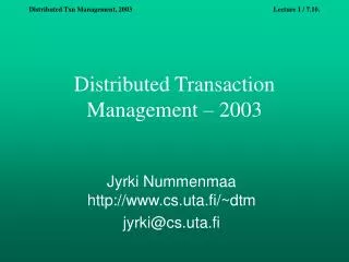
Distributed Transaction Management – 2003 Jyrki Nummenmaa http://www.cs.uta.fi/~dtm jyrki@cs.uta.fi
Coordinated universal time • Atomic clocks based on atomic oscillations are the most accurate physical clocks. • So-called Coordinated Universal Time based on atomic time is signaled from radio stations and satellites. • You can buy a receiver (maybe not more than $100, I had a look at the web) and get accuracy in the order of 0.1-10 milliseconds.
Reasons for and problems in clock synchronisation • Different clocks work at different speeds. Therefore, they need to be synchronised at times (continuously). • Message delay can not be known, but must be approximated -> perfect synchronisation can not be achieved. • Clock skew: difference in simultaneous readings. • Clock drift: divergence of clocks because of different clock speeds.
External and Internal Synchronisation • External synchronisation of clock C is synchronisation with some external source E. If |C-E|<d, then C is accurate (with respect to E) within the bound d. • Internal synchronisation is synchronisation of clocks C and C’ between themselves. If |C-C’|<d, then C and C’ agree within the bound d. C and C’ may drift from an external source, but not from each other.
Cristian’s synchronisation method • A clock at site S is synchronised with a clock at site S’ by sending a request Mr to S and receiving a time message Mt from S containing time t. • Round-trip time Tr is the time between sending Mr and receiving Mt. This is a small time and can be measured accurately. • A simple estimate: S will set its clock to t + Tr / 2.
Accuracy of Cristian’s synchronisation • Assume min is shortest time for a message to travel from S to S’ (this must be approximated). • When Mt arrives to S, the clock of S’ will read in the range [t+min, t+Tr-min]. This range has width Tr - 2min. • We set the clock of S to t + Tr/2. • -> Accuracy is plus/minus Tr / 2 -min
Problems and improvements • Problem: A single source for time. • Improvement: Poll several servers and e.g. use the fastest reply. • Problem: Faulty time servers. • Improvement: Poll several servers and use statistics.
Further improvements • Berkely time protocol: internal synchronisation with a server polling a number of slaves and using an average of estimates and sends the necessary correction to the slaves. • The Network Time Protocol: A hierarchy of servers. Top level = UTC, second level synchronises with top level and so on. More details at http://www.ntp.org.
Applications of clocks • Clocks are needed in timestamp concurrency control to generate the timestamps! • If we are satisfied with clock accuracy (and accept the clock skew) then we can use the physical clock time stamps. • If not, then logical ordering of events needs to be used.
Token-based algorithms for resource management • In the token-based algorithms, there is a token to represent the permission. • Whoever has the token, has the permission, and can pass it on. • These algorithms are more suitable to share a resource like a printer, a car park gate, etc than for a huge database. Let’s see why…
Perpetuum mobile • The token travels around (say, a ring). • When a process receives the token, it may use the resource, if it so wishes. • Then the process passes the token on. TOKEN
Token-asking algorithms • The token does not travel around if it is not needed. • When a process needs the token, it asks for it. • Requests are queued.
Analysis of token-based algorithms • Safety – ok. • Liveness – ok. • Fairness – in a way ok. • Drawbacks:- They are vulnerable to single-site failures.- Token management may be complicated and/or consume lots of resources, if there are lots of resources to be managed.
Logical order • Using physical clocks to order events is problematic, because we can not completely synchronise the clocks. • An alternative solution: use a logical (causality) order.
What kind of events we can use to compute a logical order? • If e1 happens before e2 on site S, then we write e1 <S e2. • If e1 is the sending of message m on some processor and e2 is the receiving of message m on some processor, then we write e1 <m e2.
The happens-before relation • The happens-before relation is denoted by <H. • If e1 <S e2, then e1 <H e2. • If e1 <m e2, then e1 <H e2. • If e1 <H e2 and e2 <H e3,then e1 <H e3. • If happens-before relation does not order two events, we call them concurrent.
e1 <S1 e2 e2 <S1 e3 e3 <S1 e4 e5 <S2 e6 e6 <S2 e7 e7 <S2 e8 e1 <m1 e5 e3 <m2 e6 e7 <m3 e4 Plus the transitive closure Happens-before example S1 S2 m1 e1 e5 e2 e6 m2 e3 e7 m3 e6 e4
The happens-before graph • Form a directed graph with events as vertices. • If e1 <S e2 or e1 <H e2, then there is an edge from e1 to e2. • The closure of the graph represents the happens-before relation.
Happens-before graph S1 S2 m1 e1 e1 e5 e5 e2 e6 e2 m2 e3 e7 e6 m3 e8 e4 e3 e7 e4 e8 The transitive closure represents full information on the logical order
Lamport timestamps • Initially, assing 0 to myTS. • If event e is the receipt of a m, then: Assign max(m.TS,myTS) to myTS. Add 1 to myTS. Assign myTS to e.TS. • If event e is the sending of a m, then: Add 1 to myTS. Assign myTS to both e.TS and m.TS.
Find the logical order of events. T’’ T T’ T’’’ m1 m2 m3 m4 m5 m6 m7 m8 m9
Use Lamport timestamps T’’ T T’ T’’’ m1 1 2 m2 1 m3 3 4 m4 m5 5 1 4 5 m6 6 8 7 9 m7 m8 10 12 11 m9 13 14
Lamport timestamps - properties • Lamport timestamps guarantee that if e<H e', then e.TS < e'.TS - This follows from the definition of happens-before relation by observing the path of events from e to e’. • Lamport timestamps do not guarantee that if e.TS < e'.TS, then e <H e' (why?).
Assigning vector timestamps • Initially, assign [0,...,0] to myVT. • If event e is the receipt of m, then: For i=1,...,M, assign max(m.VT[i],myVT[i]) to myVT[i]. Add 1 to myVT[self]. Assign myVT to e.VT. • If event e is the sending of m, then: Add 1 to myVT[self]. Assign myVT to both e.VT and m.VT.
Vector timestamps T3 T1 T2 T4 m1 [1,0,0,1] [1,0,0,0] m2 m3 [0,1,0,0] [1,0,0,2] [2,0,0,2] m4 [0,0,1,0] m5 [3,0,0,2] [1,0,1,3] [1,1,1,4] m6 [3,1,2,6] [3,1,1,5] [3,1,1,6] m7 [3,1,3,6] [3,2,3,8] m8 [3,1,3,7] [3,1,3,8] m9 [3,3,3,8] [3,3,3,9]
Vector timestamp order • e.VT V e'.VT, if and only if e.VT[i] e'.VT[i], 1 i M. • e.VT <V e'.VT, if and only if e.VT[i] V e'.VT[i], and e.VT e'.VT. • [0,1,2,3] [0,1,2,3] • [0,1,2,2] <[0,1,2,3] • The order of [0,1,2,3] and [1,1,2,4] is not defined, they are concurrent.
Vector timestamps - properties • Vector timestamps also guarantee that if e<H e', then e.VT < e'.VT - This follows from the definition of happens-before relation by observing the path of events from e to e’. • Vector timestamps also guarantee that if e.VT < e'.VT, then e <H e' (why?).
Deadlock - Introdcution • Centralised example: • T1 locks X on time t1. • T2 locks Y on time t2. • T1 attempts to lock Y on time t3 and gets blocked. • T2 attempts to X on time t4 and gets blocked.
Deadlock (continued) • Deadlock can occur in centralised systems. For example: • At the operating system level there can be resource contention between processes • At the transaction processing level there can be data contention between transactions. • In a poorly-designed multithread program, there can be deadlock between threads in the same process.
Distributed deadlock ”management” approaches • The approach taken by distributed systems designers to the problem of deadlock depends on the frequency with which it occurs. • Possible strategies: • Ignore it. • Detection (and recovery). • Prevention and Avoidance (by statically making deadlock structurally impossible and by allocating resources carefully). • Detect local deadlock and ignore global deadlock.
Ignore deadlocks? • If the system ignores the deadlocks, then the application programmers have to make their applications in such a way, that a timeout will force the transaction to abort and possibly re-start. • The same approach is sometimes used in the centralised world.
Distributed Deadlock Prevention and Avoidance • Some proposed techniques are not feasible in practice, like making a process request all of its resources at the start of execution. • For transaction processing systems with timestamps, the following scheme can be implemented (like in centralised world): • When a process blocks, its timestamp is compared to the timestamp of the blocking process. • The blocked process is only allowed to wait if it has a higher timestamp. • This avoids any cyclic dependency.
Wound-wait and wound-die • In the wound-wait approach, if an older process requests a lock to an item held by a younger process, it wounds the younger process and effectively kills it. • In the wait-die approach, if a younger process requests a lock to an item held by an older process, the younger process commits suicide. • Both of these approaches kill transactions blindly. There does not need to be a deadlock.
Further considerations for wound-wait and wound-die • To reduce the number of unnecessarily aborted transactions, it is possible to use the cautious waiting rule: ”You are always allowed to wait for a process, which is not waiting for another process.” • The aborted processes are re-started with their original timestamps, to guarantee liveness. • Otherwise, a transaction may not make progress if it gets aborted over and over again.
Local waits-for graphs • Each resource manager can maintain its local `waits-for' graph. • A coordinator maintains a global waits-for graph. When the coordinator detects a deadlock, it selects a victim process and kills it (thereby causing its resource locks to be released), breaking the deadlock. • Problem: The information about changes must be transmitted to the coordinator. The coordinator knows nothing about change information that is in transit. Thus, in practice, many of the deadlocks that it thinks it has detected will be what they call in the trade `phantom deadlocks'.
Waits-for graph • Centralised: a cycle in the waits-for graph means a deadlock T1 T2 T3
Local vs Global • Distributed: collect the local graphs and create a global waits-for graph. T1 T1 T2 T1 T2 T3 T3 T3 Site 1 Site 2 Global waits-for graph
Global state • We assume that between each pair (Si,Sj) of sites there is a reliable order-preserving communication channel C{i,j}, whose contents is a list of messages L{i,j}=m1(i,j),m2(i,j), ..., mk(i,j). • Let L={L{i,j}} be the collection of all message lists and K the collection of all local states. We say that the pair G=(K,L) is the global state of the system.
Consistent cut • We say that a global state G=(K,L) is a consistent cut, if for each event e in G, G contains all events e’ such that e’ <H e. • That is, there are no events missing from G such that they have happened before e.
Which lines cut a consistent cut? T’’ T T’ T’’’ m1 m2 m3 m4 m5 m6 m7 m8 m9
Distributed snapshots • We denote the state of Site i by Si. • A state of a site at one time is called a snapshot. • There is no way we can take the snapshots simultaneously. If we could, that would solve the deadlock detection. • Therefore, we want to create a snapshot that reflects a consistent cut.
Computing a distributed snapshot / Assumptions and requirements • If we form a graph with sites as nodes and communication channels as edges, we assume that the graph is connected. • Neither channels nor processes fail. • Any site may initiate snapshot computation. • There may be several simultaneous snapshot computations.
Computing a distributed snapshot / 1 • As a site Sj initiates snapshot collection, it records its state and sends snapshot token to all sites it communicates with.
Computing a distributed snapshot / 2 • If a site Si, i j, receives a snapshot token for the first time, and it receives it from Sk, it does the following: 1. Stops processing messages. 2. Makes L(k,i) the empty list. 3. Records its state. 4. Sends a snapshot token to all sites it communicates with. 5. Continues to process messages.
Computing a distributed snapshot / 3 • If a site Si receives a snapshot token from Sk and it has received a snaphost token also earlier on or i = j, then the list L(k,i) is the list of messages Si has received from Sk after recording its state.
Distributed snapshot example Assume connection set { (S1,S2), (S2,S3), (S3,S4) } S3 S1 S2 S4 snap snap m2 m3 m1 snap snap snap m4 m5 snap L(1,2) = { m1 }, L(2,3) = {}, L(3,4) = { m3, m4 }. Effects of m2 are included in the state of S4. Message m5 takes place entirely after the snapshot computation.