Download

1 / 20
200 likes | 287 Views
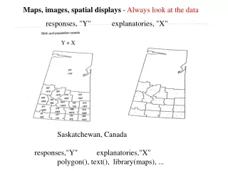
Maps, images, spatial displays - Always look at the data responses, "Y" explanatories, "X". Y + X. Saskatchewan, Canada responses,"Y" explanatories,"X" polygon(), text(), library(maps),. Examples from the news Costa Concordia - Giglio.

E N D
Maps, images, spatial displays - Always look at the data responses, "Y" explanatories, "X" Y + X Saskatchewan, Canada responses,"Y" explanatories,"X" polygon(), text(), library(maps), ...
Examples from the news Costa Concordia - Giglio
Coal used for electricity circles(), polygon() NY Times 01/27/09
Spatial process data. (s,t): geographic coordinates, e.g. (latitude, longitude), (x-coord,y-coord) y(s,t): real-valued e.g. available for s=0,...,S-1; t=0,...,T-1 (s,t) in A
Height of 500mb surface S=64, T=32 1200 GMT January 1, 1986 data based on many observations, interpolated to grid display by contours over a world map
overall mean subtracted map(), lines(), 2
Ocean currents red: eastward blue: westward http://www.oscar.noaa.gov/ map(), arrows()
Stacking. Galton - photos of faces electron micrographs crystal, purple membrane symmetries 160 "units" j=1160 yj(s,t)/160 stacking via FFT fft(), lines()
micrographs not stacked and stacked J=1 J=160
Data may be aggregate, e.g. over polygons coordinates of vertices choropleth plot: a thematic map in which areas are shaded map(), polygon() computational geometry, point in polygon library(splancs) Saskatchewan births, counts, rates
perspective plot persp() hidden lines
Contouring. Contour line, , (a function of two variables), is a curve connecting points where the function has the same value. Smooth function f: R2 R c: value f-1 (c) = x,y There may be more than one component
One method. Suppose f(s,t) available for a regular grid Suupose wish f-1(c) Pick an edge, AB, of a pixel I. It will be intercepted if min{f(A),f(B)}cmax{f(A),f(B)} using this can learn all edges intercepted II. If one edge of a cell is intercepted, so is another one search in order E-S-W-N III. Get intersection coordinates by interpolation connect by line IV. Move to pertinent adjacent cell and continue
Line process - set of lines {l1 , l2 , ls ,...} Point process {(p(l1),(l1)),(p(l2),(l2)),...} p: distance : angle
Tesselation #{cells completely in set A} polygon()