Download
1 / 58
580 likes | 747 Views
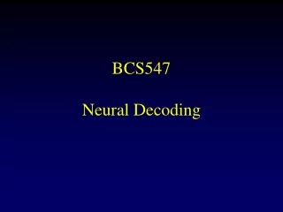
BCS547 Neural Decoding. Population Code. 100. 100. s?. 80. 80. 60. 60. Activity. Activity. 40. 40. 20. 20. 0. 0. -100. 0. 100. -100. 0. 100. Direction (deg). Preferred Direction (deg). Tuning Curves. Pattern of activity (r).

E N D
Population Code 100 100 s? 80 80 60 60 Activity Activity 40 40 20 20 0 0 -100 0 100 -100 0 100 Direction (deg) Preferred Direction (deg) Tuning Curves Pattern of activity (r)
Estimation theory: come up with a single value estimate from r Nature of the problem In response to a stimulus with unknown orientation s, you observe a pattern of activity r. What can you say about s given r? Bayesian approach: recover p(s|r) (the posterior distribution)
100 80 60 Activity 40 20 0 -100 0 100 Preferred Direction (deg) Pattern of activity (r) Maximum Likelihood 100 80 60 Activity 40 20 0 -100 0 100 Direction (deg) Tuning Curves
100 80 60 Activity 40 20 0 -100 0 100 Preferred Direction (deg) Maximum Likelihood Template
100 80 60 40 20 -100 0 100 Maximum Likelihood Activity 0 Template Preferred Direction (deg)
100 80 60 40 20 -100 0 100 Maximum Likelihood Activity 0 Preferred Direction (deg)
Noise distribution Maximum Likelihood The maximum likelihood estimate is the value of s maximizing the likelihood p(r|s). Therefore, we seek such that:
P(ai|q=-60) P(ri|s=-60) P(ri|s=0) Activity distribution
Noise distribution Maximum Likelihood The maximum likelihood estimate is the value of s maximizing the likelihood p(s|r). Therefore, we seek such that: is unbiased and efficient.
Decoder Encoder (nervous system) 100 80 60 40 20 0 -100 0 100 Preferred orientation Estimation Theory Activity vector: r
r1 Trial 1 Encoder (nervous system) Decoder Encoder (nervous system) Decoder Decoder Encoder (nervous system) r2 Trial 2 100 80 60 40 20 0 r200 -100 0 100 Trial 200 Preferred retinal location 100 80 100 80 60 60 40 40 20 20 0 -100 0 100 Preferred retinal location 0 -100 0 100 Preferred retinal location
Estimation Theory Decoder Encoder (nervous system) If , the estimate is said to be unbiased 100 80 If is as small as possible, the estimate is said to be efficient 60 40 20 0 -100 0 100 Preferred orientation Activity vector: r
Estimation theory • A common measure of decoding performance is the mean square error between the estimate and the true value • This error can be decomposed as:
Efficient Estimators The smallest achievable variance for an unbiased estimator is known as the Cramer-Rao bound, sCR2. An efficient estimator is such that In general :
Fisher Information and it is equal to: Fisher information is defined as: where p(r|s) is the distribution of the neuronal noise.
Large slope is good! The more neurons, the better! Small variance is good! Fisher Information • For one neuron with Poisson noise • For n independent neurons :
Fisher Information and Tuning Curves • Fisher information is maximum where the slope is maximum • This is consistent with adaptation experiments
Fisher Information • In 1D, Fisher information decreases as the width of the tuning curves increases • In 2D, Fisher information does not depend on the width of the tuning curve • In 3D and above, Fisher information increases as the width of the tuning curves increases • WARNING: this is true for independent gaussian noise.
Ideal observer The discrimination threshold of an ideal observer, ds, is proportional to the variance of the Cramer-Rao Bound. In other words, an efficient estimator is an ideal observer.
An ideal observer is an observer that can recover all the Fisher information in the activity (easy link between Fisher information and behavioral performance) • If all distributions are gaussians, Fisher information is the same as Shannon information.
Decoder Encoder (nervous system) 100 80 60 40 20 0 -100 0 100 Preferred orientation Estimation theory Activity vector: r Other examples of decoders
Voting Methods Optimal Linear Estimator
Linear Estimators X and Y must be zero mean Trust cells that have small variances and large covariances
Voting Methods Optimal Linear Estimator
Linear in ri/Sjrj Weights set to si Voting Methods Optimal Linear Estimator Center of Mass
Center of Mass/Population Vector • The center of mass is optimal (unbiased and efficient) iff: The tuning curves are gaussian with a zero baseline, uniformly distributed and the noise follows a Poisson distribution • In general, the center of mass has a large bias and a large variance
Linear in ri Weights set to Pi Nonlinear step Voting Methods Optimal Linear Estimator Center of Mass Population Vector
P riPi s Population Vector
Population Vector Typically, Population vector is not the optimal linear estimator.
Population Vector • Population vector is optimal iff: The tuning curves are cosine, uniformly distributed and the noise follows a normal distribution with fixed variance • In most cases, the population vector is biased and has a large variance • The variance of the population vector estimate does not reflect Fisher information
Population Vector Population vector CR bound Population vector should NEVER be used to estimate information content!!!! The indirect method is prone to severe problems…
100 80 60 40 20 -100 0 100 Maximum Likelihood Activity 0 Preferred Direction (deg)
Distance measure: Template matching Maximum Likelihood If the noise is gaussian and independent Therefore and the estimate is given by:
Gradient descent for ML • To minimize the likelihood function with respect to s, one can use a gradient descent technique in which s is updated according to:
Data point with small variance are weighted more heavily Gaussian noise with variance proportional to the mean If the noise is gaussian with variance proportional to the mean, the distance being minimized changes to:
Poisson noise If the noise is Poisson then And :
ML and template matching Maximum likelihood is a template matching procedure BUT the metric used is not always the Euclidean distance, it depends on the noise distribution.
prior distribution over s likelihood of s prior distribution over r posterior distribution over s Bayesian approach We want to recover p(s|r). Using Bayes theorem, we have:
Bayesian approach What is the likelihood of s, p(r| s)?It is the distribution of the noise… It is the same distribution we used for maximum likelihood.
Bayesian approach • The prior p(s) correspond to any knowledge we may have about s before we get to see any activity. • Ex: prior for smooth and slow motions
Bayesian approach Once we have p(s|r), we can proceed in two different ways. We can keep this distribution for Bayesian inferences (as we would do in a Bayesian network) or we can make a decision about s. For instance, we can estimate s as being the value that maximizes p(s|r),This is known as the maximum a posteriori estimate (MAP). For flat prior, ML and MAP are equivalent.
Bayesian approach Limitations: the Bayesian approach and ML require a lot of data (estimating p(r|s) requires at least n+(n-1)(n-1)/2 parameters for multivariate gaussian)… Alternative: 1- Naïve Bayes: assume independence and hope for the best 2- Use clever method for fitting p(r|s). 3- Estimate p(s|r)directly using a nonlinear estimate. 4- hope the brain uses likelihood functions that have only N free parameters, e.g., the exponential family with linear sufficient statistics
Bayesian approach:logistic regression Example: Decoding finger movements in M1. On each trial, we observe 100 cells and we want to know which one of the 5 fingers is being moved. P(F5|r) 1 0 5 categories 1 2 3 4 5 g(x) … 100 input units 1 2 3 100 r
Bayesian approach:logistic regression Example: 5N free parameters instead of O(N2) P(F5|r) 1 0 5 categories 1 2 3 4 5 s … 100 input units 1 2 3 100 r
Probability of no movement Probability of flexion Probability of extension Digit 1 Digit 2 Digit 3 Digit 4 Digit 5 Wrist Softmax W Activity of the N M1 neurons Bayesian approach:multinomial distributions Example: Decoding finger movements in M1. Each finger can take 3 mutually exclusive states: no movement, flexion, extension.