Download
1 / 47
550 likes | 832 Views
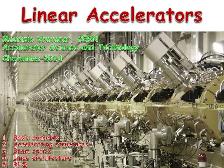
Linear Accelerators. Maurizio Vretenar, CERN Accelerator Science and Technology Chavannes 2014. Basic concepts Accelerating structures Beam optics Linac architecture RFQ. 1. Introduction: main concepts, building blocks, synchronicity. Why Linear Accelerators.

E N D
Linear Accelerators Maurizio Vretenar, CERNAccelerator Science and Technology Chavannes 2014 • Basic concepts • Accelerating structures • Beam optics • Linac architecture • RFQ
1. Introduction:main concepts, building blocks, synchronicity 2
Why Linear Accelerators Linear Accelerators are used for: • Low-Energy acceleration (injectors to synchrotrons or stand-alone): for protons and ions, linacs can be synchronous with the RF fields in the range where velocity increases with energy. When velocity is ~constant, synchrotrons are more efficient (multiple crossings instead of single crossing). Protons : b = v/c =0.51 at 150 MeV, 0.95 at 2 GeV. • High-Energy acceleration in the case of: • Production of high-intensity proton beams,in comparison with synchrotrons,linacs can go to higher repetition rate, are less affected by resonances and instabilities and have more distributed beam losses.Higher injection energy from linacs to synchrotrons leads to lower space charge effects in the synchrotron and allows increasing the beam intensity. • High energy linear colliders for leptons, where the main advantage is the absence of synchrotron radiation. 3
Proton and Electron Velocity protons, classical mechanics b2=(v/c)2 as function of kinetic energy T for protons and electrons. electrons Classic (Newton) relation: Relativistic (Einstein) relation: “Newton” region protons “Einstein” region • Protons(rest energy 938.3 MeV): follow “Newton” mechanics up to some tens ofMeV (Dv/v < 1% for W < 15 MeV) then slowly become relativistic (“Einstein”). From the GeV range velocity is nearly constant (v~0.95c at 2 GeV) linacs can cope with the increasing particle velocity, synchrotrons cover the range where v nearly constant. • Electrons (rest energy 511 keV, 1/1836 of protons): relativistic from the keV range (v~0.1c at 2.5 keV) then increasing velocity up to the MeV range (v~0.95c at 1.1 MeV) v~c after few meters of acceleration (typical gradient 10 MeV/m). 4
Linear and circular accelerators Synchronism conditions d=bl/2=variable d=2pR=constant accelerating gaps d accelerating gap d Linear accelerator: Particles accelerated by a sequence of gaps (all at the same RF phase). Distance between gaps increases proportionally to the particle velocity, to keep synchronicity. Used in the range where b increases. “Newton” machine Circular accelerator: Particles accelerated by one (or more) gaps at given positions in the ring. Distance between gaps is fixed. Synchronicity only for b~const, or varying (in a limited range!) the RF frequency. Used in the range where b is nearly constant. “Einstein” machine 5
Basic linear accelerator structure RF cavity Focusing magnet B-field DC particle injector bunching section E-field ? d Protons: energy ~20-100 keV b= v/c ~ 0.01 Accelerating gap: E = E0 cos (wt + f) en. gain DW = eV0Tcosf Acceleration the beam has to pass in each cavity on a phase f near the crest of the wave The beam must to be bunched at frequency w distance between cavities and phase of each cavity must be correlated Phase change from cavity i to i+1 is For the beam to be synchronous with the RF wave (“ride on the crest”) phase must be related to distance by the relation: … and on top of acceleration, we need to introduce in our “linac” some focusing elements 6 … and on top of that, we will couple a number of gaps in an “accelerating structure”
Accelerating structure architecture When b increases during acceleration, either the phase difference between cavities Dfmust decrease or their distance d must increase. d = const. f variable d Individual cavities – distance between cavities constant, each cavity fed by an individual RF source, phase of each cavity adjusted to keep synchronism, used for linacs required to operate with different ions or at different energies. Flexible but expensive! Better, but 2 problems: create a “coupling”; create a mechanical and RF structure with increasing cell length. f = const. d variable d bl Coupled cell cavities - a single RF source feeds a large number of cells (up to ~100!) - the phase between adjacent cells is defined by the coupling and the distance between cells increases to keep synchronism . Once the geometry is defined, it can accelerate only one type of ion for a given energy range. Effective but not flexible.
Case 1: a single-cavity linac The goal is flexibility: acceleration of different ions (e/m) at different energies need to change phase relation for each ion-energy RF cavity focusing solenoid HIE-ISOLDE linac (in construction at CERN - superconducting) Post-accelerator of radioactive ions 2 sections of identical equally spaced cavities Quarter-wave RF cavities, 2 gaps 12 + 20 cavities with individual RF amplifiers, 8 focusing solenoids Energy 1.2 10 MeV/u, accelerates different A/m beam 8
Case 2 : a Drift Tube Linac d 10 MeV, b = 0.145 50 MeV, b = 0.31 Tank 2 and 3 of the new Linac4 at CERN: 57 coupled accelerating gaps Frequency 352.2 MHz, l = 85 cm Cell length (d=bl) from 12.3 cm to 26.4 cm (factor 2 !). 9
Case 3 (intermediate): the Linac4 PIMS structure Between these 2 “extremes” there are “intermediate” cases: a) single-gap cavities are expensive and b) structures with each cell matched to the beta profile are mechanically complicated → as soon as the increase of beta with energy becomes smaller we can accept a small phase error and allow short sequences of identical cells. PIMS: cells have same length inside a cavity (7 cells) but increase from one cavity to the next. At high energy (>100 MeV) beta changes slowly and phase error remains small. 160 MeV, 155 cm Focusing quadrupoles between cavities 100 MeV, 128 cm PIMS range 10
Multi-gap coupled-cell cavities (for protons and ions) Between the 2 extreme cases (array of independently phased single-gap cavities / single long chain of coupled cells with lengths matching the particle beta) there can be a large number of variations (number of gaps per cavity, length of the cavity, type of coupling) each optimized for a certain range of energy and type of particle. The goal of this lecture is to provide the background to understand the main features of these different structures… DTL SCL CH PIMS CCDTL 11
(Proton) linac building blocks HV AC/DC power converter AC to DC conversion efficiency ~90% Main oscillator DC to RF conversion efficiency ~50% RF feedback system High power RF amplifier (tube or klystron) RF to beam voltage conversion efficiency = SHUNT IMPEDANCE ZT2 ~ 20 - 60 MW/m DC particle injector buncher ion beam, energy W magnet powering system vacuum system water cooling system LINAC STRUCTURE accelerating gaps + focusing magnets designed for a given ion, energy range, energy gain 12
Electron linacs In an electron linac velocity is ~ constant. To use the fundamental accelerating mode cell length must be d = bl / 2. the linac structure will be made of a sequence of identical cells. Because of the limits of the RF source, the cells will be grouped in cavities operating in travelling wave mode. 13 Pictures from K. Wille, The Physics of Particle Accelerators
Coupling accelerating cells 1. Magnetic coupling: open “slots” in regions of high magnetic field B-field can couple from one cell to the next 2. Electric coupling: enlarge the beam aperture E-field can couple from one cell to the next How can we couple together a chain of n accelerating cavities ? The effect of the coupling is that the cells no longer resonate independently, but will have common resonances with well defined field patterns. 16
Linac cavities as chains of coupled resonators What is the relative phase and amplitude between cells in a chain of coupled cavities? R A linear chain of accelerating cells can be represented as a chain of resonant circuits magnetically coupled. Individual cavity resonating at w0 frequenci(es) of the coupled system ? Resonant circuit equation for circuit i (R0, M=k√L2): M M L L L Ii L C Dividing both terms by 2jwL: General response term, (stored energy)1/2, can be voltage, E-field, B-field, etc. Contribution from adjacent oscillators General resonance term 17
The Coupled-system Matrix A chain of N+1 resonators is described by a (N+1)x(N+1) matrix: or This matrix equation has solutions only if • Eigenvalue problem! • System of order (N+1) in w only N+1 frequencies will be solution of the problem (“eigenvalues”, corresponding to the resonances) a system of N coupled oscillators has N resonance frequencies an individual resonance opens up into a band of frequencies. • At each frequency wi will correspond a set of relative amplitudes in the different cells (X0, X2, …, XN): the “eigenmodes” or “modes”. 18
Modes in a linear chain of oscillators We can find an analytical expression for eigenvalues (frequencies) and eigenvectors (modes): the index q defines the number of the solution is the “mode index” Frequencies of the coupled system : • Each mode is characterized by a phase pq/N. Frequency vs. phase of each mode can be plotted as a “dispersion curve” w=f(f): • each mode is a point on a sinusoidal curve. • modes are equally spaced in phase. w0/√1-k w0 w0/√1+k p 0 p/2 The “eigenvectors = relative amplitude of the field in the cells are: STANDING WAVE MODES, defined by a phase pq/N corresponding to the phase shift between an oscillator and the next one pq/N=F is the phase difference between adjacent cells that we have introduces in the 1st part of the lecture. 19
Example: Acceleration on the normal modes of a 7-cell structure 0 w = w0/√1+k 0 (or 2p) mode, acceleration if d = bl Intermediate modes p/2 w = w0 p/2 mode, acceleration if d = bl/4 … w = w0/√1-k p 20 p mode, acceleration if d = bl/2, Note: Field always maximum in first and last cell!
Practical linac accelerating structures Note: our equations depend only on the cell frequency w0, not on the cell length d !!! As soon as we keep the frequency of each cell constant, we can change the cell length following any acceleration (b) profile! Example: The Drift Tube Linac (DTL) Chain of many (up to 100!) accelerating cells operating in the 0 mode. The ultimate coupling slot: no wall between the cells! Each cell has a different length, but the cell frequency remains constant “the EM fields don’t see that the cell length is changing!” d (L , C↓) LC ~ const w0~ const 21
The Drift Tube Linac (DTL) Standing wave linac structure for protons and ions, b=0.1-0.5, f=20-400 MHz Drift tubes are suspended by stems (no net RF current on stem) Coupling between cells is maximum (no slot, fully open !) The 0-mode allows a long enough cell (d=bl) to house focusing quadrupoles inside the drift tubes! E-field B-field 22
The Linac4 DTL DTL tank 1 fully equipped: focusing by small permanent quadrupoles inside drift tubes. 352 MHz frequency Tank diameter 500mm 3 resonators (tanks) Length 19 m 120 Drift Tubes Energy 3 MeV to 50 MeV Beta 0.08 to 0.31 cell length (bl) 68mm to 264mm factor 3.9 increase in cell length beam 23
Shunt impedance How to choose the best linac structure? Main figure of merit is the power efficiency = shunt impedance Ratio between energy gain (square) and power dissipation, is a measure of the energy efficiency of a structure. Depends on beta, energy and mode of operation. But the choice of the best accelerating structure for a certain energy range depends as well on beam dynamics and on construction cost. Comparison of shunt-impedances for different low-beta structures done in 2005-08 by the “HIPPI” EU-funded Activity. In general terms, a DTL-like structure is preferred at low-energy, and p-mode structures at high-energy. CH is excellent at very low energies (ions). 24
Multi-gap Superconducting linac structures (elliptical) Standing wave structures for particles at b>0.5-0.7, widely used for protons (SNS, etc.) and electrons (ILC, etc.) f=350-700 MHz (protons), f=350 MHz – 3 GHz (electrons) Chain of cells electrically coupled, large apertures (ZT2 not a concern). Operating in p-mode, cell length bl/2 Input coupler placed at one end. 25
The superconducting zoo Spoke (low beta) [FZJ, Orsay] QWR (low beta) [LNL, etc.] CH (low/medium beta) [IAP-FU] 10 gaps 2 gaps Re-entrant [LNL] 4 gaps HWR (low beta) [FZJ, LNL, Orsay] 4 to 7 gaps 2 gaps 1 gap Superconducting structure for linacs can have a small number of gaps → used for low and medium beta. Elliptical structures with more gaps (4 to 7) are used for medium and high beta. Elliptical cavities [CEA, INFN-MI, CERN, …] 26
Traveling wave accelerating structures (electrons) What happens if we have an infinite chain of oscillators? becomes (N∞) becomes (N∞) All modes in the dispersion curve are allowed, the original frequency degenerates into a continuous band. The field is the same in each cell, there are no more standing wave modes only “traveling wave modes”, if we excite the EM field at one end of the structure it will propagate towards the other end. w0/√1-k w0 w0/√1+k 0 p/2 p But: our dispersion curve remains valid, and defines the velocity of propagation of the travelling wave, vf = wd/F For acceleration, the wave must propagate at vf= c for each frequency w and cell length d we can find a phase F where the apparent velocity of the wave vf is equal to c 27
Traveling wave accelerating structures How to “simulate” an infinite chain of resonators? Instead of a singe input, exciting a standing wave mode, use an input + an output for the RF wave at both ends of the structure. w vph= c beam “Disc-loaded waveguide” or chain of electrically coupled cells characterized by a continuous band of frequencies. In the chain is excited a “traveling wave mode” that has a propagation velocity vph= w/k given by the dispersion relation. For a given frequency w,vph= c and the structure can be used for particles traveling at b=1 The “traveling wave” structure is the standard linac for electrons from b~1. • Can not be used for protons at v<c: 1. constant cell length does not allow synchronism 2. structures are long, without space for transverse focusing 28
Longitudinal dynamics • Ions are accelerated around a (negative = linac definition) synchronous phase. • Particles around the synchronous one perform oscillations in the longitudinal phase space. • Frequency of small oscillations: • Tends to zero for relativistic particles g>>1. • Note phase damping of oscillations: At relativistic velocities phase oscillations stop, and the beam is compressed in phase around the initial phase. The crest of the wave can be used for acceleration. 30
Transverse dynamics - Space charge • Large numbers of particles per bunch ( ~1010 ). • Coulomb repulsion between particles (space charge) plays an important role and is the main limitation to the maximum current in a linac. • But space charge forces ~ 1/g2 disappear at relativistic velocity Force on a particle inside a long bunch with density n(r) traveling at velocity v: B E 31
Transverse dynamics - RF defocusing • RF defocusing experienced by particles crossing a gap on a longitudinally stable phase. Increasing field means that the defocusing effect going out of the gap is stronger than the focusing effect going in. • In the rest frame of the particle, only electrostatic forces no stable points (maximum or minimum) radial defocusing. • Lorentz transformation and calculation of radial momentum impulse per period (from electric and magnetic field contribution in the laboratory frame): Bunch position at max E(t) • Transverse defocusing~ 1/g2 disappears at relativistic velocity 32
Focusing Defocusing forces need to be compensated by focusing forces → alternating gradient focusing provided by quadrupoles along the beam line. A linac alternates accelerating sections with focusing sections. Options are: one quadrupole (singlet focusing), two quadrupoles (doublet focusing) or three quadrupoles (triplet focusing). Focusing period=length after which the structure is repeated (usually as Nbl). The accelerating sections have to match the increasing beam velocity → the basic focusing period increases in length (but the beam travel time in a focusing period remains constant). The maximum allowed distance between focusing elements depends on beam energy and current and change in the different linac sections (from only one gap in the DTL to one or more multi-cell cavities at high energies). 33
Transverse beam equilibrium in linacs The equilibrium between external focusing force and internal defocusing forces defines the frequency of beam oscillations. Oscillations are characterized in terms of phase advance per focusing periodstor phase advance per unit lengthkt. Ph. advance = Ext. quad focusing - RF defocusing - space charge q=charge G=quad gradient l=length foc. element f=bunch form factor r0=bunch radius l=wavelength … Approximate expression valid for: F0D0 lattice, smooth focusing approximation, space charge of a uniform 3D ellipsoidal bunch. A “low-energy” linac is dominated by space charge and RF defocusing forces !! Phase advance per period must stay in reasonable limits (30-80 deg), phase advance per unit length must be continuous (smooth variations) at low b, we need a strong focusing term to compensate for the defocusing, but the limited space limits the achievable G and l needs to use short focusing periods N bl. Note that the RF defocusing term f sets a higher limit to the basic linac frequency (whereas for shunt impedance considerations we should aim to the highest possible frequency, Z √f). 34 34
Phase advance – an example Beam optics of the Linac4 Drift Tube Linac (DTL): 3 to 50 MeV, 19 m, 108 focusing quadrupoles (permanent magnets). Oscillations of the beam envelope (coordinates of the outermost particle) along the DTL (x, y, phase) Corresponding phase advance per period • Design prescriptions: • Tranverse phase advanceatzerocurrentalwayslessthan 90°. • Smooth variation of the phase advance. • Avoidresonnances (seenextslide). 35
Focusing periods Focusing usually provided by quadrupoles. Need to keep the phase advance in the good range, with an approximately constant phase advance per unit length → The length of the focusing periods has to change along the linac, going gradually from short periods in the initial part (to compensate for high space charge and RF defocusing) to longer periods at high energy. For Protons(high beam current and high space charge), distance between two quadrupoles (=1/2 of a FODO focusing period): - blin the DTL, from ~70mm (3 MeV, 352 MHz) to ~250mm (40 MeV), - can be increased to 4-10bl at higher energy (>40 MeV). - longer focusing periods require special dynamics (example: the IH linac). For Electrons (no space charge, no RF defocusing): focusing periods up to several meters, depending on the required beam conditions. Focusing is mainly required to control the emittance. 36
Architecture: cell length, focusing period EXAMPLE: the Linac4 project at CERN. H-, 160 MeV energy, 352 MHz. A 3 MeV injector + 22 multi-cell standing wave accelerating structures of 3 types DTL, 3-50 MeV: every cell is different, focusing quadrupoles in each drift tube, 0-mode CCDTL, 50-100 MeV: sequences of 2 identical cells, quadrupoles every 3 cells, 0 and p/2 mode PIMS, 100-160 MeV: sequences of 7 identical cells, quadrupoles every 7 cells, p/2 mode Two basic principles to remember: 1. As beta increases, phase error between cells of identical length becomes small we can have short sequences of identical cells (lower construction costs). 2. As beta increases, the distance between focusing elements can increase. Injector 38
Linac architecture: the frequency approximate scaling laws for linear accelerators: • RF defocusing (ion linacs) ~ frequency • Cell length (=bl/2) ~ (frequency)-1 • Peak electric field ~ (frequency)1/2 • Shunt impedance (power efficiency) ~ (frequency)1/2 • Accelerating structure dimensions ~ (frequency)-1 • Machining tolerances ~ (frequency)-1 • Higher frequencies are economically convenient (shorter, less RF power, higher gradients possible) but the limitation comes from mechanical precision required in construction (tight tolerances are expensive!) and beam dynamics for ion linacs. • The main limitation to the initial frequency (RFQ) comes from RF defocusing (~ 1/(lb2g2) – 402 MHz is the maximum achievable so far for currents in the range of tens of mA’s. • High-energy linacs have one or more frequency jumps (start 200-400 MHz, first jump to 400-800 MHz, possible a 3rd jump to 600-1200 MHz): compromise between focusing, cost and size. 39
Linac architecture: superconductivity • Advantages of Superconductivity: • - Much smaller RF system (only beam power) → prefer low current/long pulse • Larger aperture (lower beam loss). • Lower operating costs (electricity consumption). • Higher gradients (thanks to cleaning procedures) • Disadvantages of Superconductivity: • - Need cryogenic system (in pulsed machines, size dominated by static loss → prefer low repetition frequency or CW to minimize filling time/beam time). • In proton linacs, need cold/warm transitions to accommodate quadrupoles → becomes more expensive at low energy (short focusing periods). • Individual gradients difficult to predict (large spread) → for protons, need large safety margin in gradient at low energy. • Conclusions: • 1. Superconductivity gives a large advantage in cost at high energy (protons)/ high duty cycle. • 2. At low proton energy / low duty cycle superconducting sections are expensive. 40
The Radio Frequency Quadrupole (RFQ) At low proton (or ion) energies, space charge defocusing is high and quadrupole focusing is not very effective, cell length becomes small conventional accelerating structures (Drift Tube Linac) are very inefficient use a (relatively) new structure, the Radio Frequency Quadrupole. ~1-3m RFQ = Electric quadrupole focusing channel + bunching + acceleration 42
RFQ properties - 1 1. Four electrodes (vanes) between which we excite an RF Quadrupole mode (TE210) Electric focusing channel, alternating gradient with the period of the RF. Note that electric focusing does not depend on the velocity (ideal at low b!) + − − 2. The vanes have a longitudinal modulation with period = bl this creates a longitudinal component of the electric field. The modulation corresponds exactly to a series of RF gaps and can provide acceleration. + − + Opposite vanes (180º) Adjacent vanes (90º) 43
RFQ properties - 2 3. The modulation period (distance between maxima) can be slightly adjusted to change the phase of the beam inside the RFQ cells, and the amplitude of the modulation can be changed to change the accelerating gradient we can start at -90º phase (linac) with some bunching cells, progressively bunch the beam (adiabatic bunching channel), and only in the last cells switch on the acceleration. An RFQ has 3 basic functions: Adiabatically bunching of the beam. Focusing, on electric quadrupole. Accelerating. Longitudinal beam profile of a proton beam along the CERN RFQ2: from a continuous beam to a bunched accelerated beam in 300 cells. 44
Peeping into an RFQ… Looking from the RF port into the new CERN RFQ (Linac4, 2011) 45
The Linac4 RFQ Energy 45 keV – 3 MeV, length 3 m, voltage 78 kV, RF power 700 kW Completed September 2012, beam commissioning on the Test Stand in March 2013 Compact design, high reliability. The Linac4 RFQ not only focuses and accelerates the beam as required, but so far it does it in a stable, reliable and reproducible way!
Linac Bibliography 1. Reference Books: T. Wangler, Principles of RF Linear Accelerators (Wiley, New York, 1998). P. Lapostolle, A. Septier (editors), Linear Accelerators (Amsterdam, North Holland, 1970). I.M. Kapchinskii, Theory of resonance linear accelerators (Harwood, Chur, 1985). K. Wille, The physics of particle accelerators (Oxford Press, Oxford, 2001). 2. General Introductions to linear accelerators M. Puglisi, The Linear Accelerator, in E. Persico, E. Ferrari, S.E. Segré, Principles of Particle Accelerators (W.A. Benjamin, New York, 1968). P. Lapostolle, Proton Linear Accelerators: A theoretical and Historical Introduction, LA-11601-MS, 1989. P. Lapostolle, M. Weiss, Formulae and Procedures useful for the Design of Linear Accelerators, CERN- PS-2000-001 (DR), 2000. P. Lapostolle, R. Jameson, Linear Accelerators, in Encyclopaedia of Applied Physics (VCH Publishers, New York, 1991). 3. CAS Schools S. Turner (ed.), CAS School: Cyclotrons, Linacs and their applications, CERN 96-02 (1996). M. Weiss, Introduction to RF Linear Accelerators, Fifth General Accelerator Physics Course, CERN-94-01. N. Pichoff, Introduction to RF Linear Accelerators, Basic Course on Gen. Accelerator Physics, CERN-2005-04. M. Vretenar, Differences between electron and ion linacs, Small Accelerators, CERN-2006-012. M. Vretenar, Low-beta Structures, RF for Accelerators, CERN-2011-007. M. Vretenar, LinearAccelerators, High Power Hadron Machines, CERN-2013-01. M. Vretenar, The Radio Frequency Quadrupole, High Power Hadron Machines, CERN-2013-01. 47