Download
1 / 40
410 likes | 542 Views
Chapter 6: Costs of Production. Learning Objectives. Define and explain the differences between accounting profit and economic profit. Understand the law of diminishing returns. Discuss the various production costs that firms face.

E N D
Learning Objectives • Define and explain the differences between accounting profit and economic profit. • Understand the law of diminishing returns. • Discuss the various production costs that firms face. • Determine a firm’s profit maximizing decision in the short run. • Describe a firm’s shutdown decision. • Understand production and costs in the long run.
Profits • Any Firm has one main goal: maximize its profit • What does exactly profit mean? • We distinguish 3 types of profits • Accounting profit • Economic profit or excess profit • Normal profit
Accounting Profit • Most common profit idea Accounting profit = total revenue – explicit costs • Explicit costs are payments firms make to purchase • Resources (labor, land, etc.) and • Products from other firms • Easy to compute • Easy to compare across firms
Economic Profit • Economic profit is the difference between a firm's total revenue and the sum of its explicit and implicit costs • Economic profit = total revenue – explicit costs – implicit costs • Economic profit = accounting profit – implicit costs • Implicit costs are the opportunity cost of the resources supplied by the firm's owners • Difficult to measure
Accounting and Economic Profit: Example • Assume firm • Total revenue = $400,000 • Explicit costs = workers’ salaries = $250,000 • Accounting profit = $400,000 - $250,000 = $150,000 • Firm’s implicit costs = $100,000 • Economic profit = $150,000 - $100,000 • Economic profit < Accounting profit • Accounting profit – Economic profit = Normal profit • Normal profit = opportunity cost of the resources used by the firm
Three Kinds of Profit Total Revenue Total Revenue = Explicit Costs + Accounting Profit Explicit Costs Explicit Costs Accounting Profit EconomicProfit = Accounting Profit – Normal Profit Normal Profit Economic Profit
Economic Profits Guide Decisions • Kamal is a corn farmer living in Turkey • Kamal’s decision: keep farming or quit? • Quit farming and earn $11,000 per year working retail • Explicit farm costs are $10,000 (including $6,000 as rent) • Total revenue is $22,000 • Kamal should stick with farming because EP > 0 • If revenue fell below $21,000, Kamal should quit
Owned Inputs • What if Kamal inherits the land? • Rent for the farm land is $6,000 of the $10,000 in explicit costs • His rent payments become an implicit cost • Kamal should abandon farming because EP < 0
Production Ideas • Production converts inputs into outputs • Many different ways to produce the same product • Technology is a recipe for production • A factor of production is an input used in the production of a good or a service • Examples are land, labor, capital, and entrepreneurship • The short run is the period of time when at least one of the firm's factors of production is fixed • The long run is the period of time in which all inputs are variable
Production: Short and Long Run • Every firm faces the following question: how much to produce? • Assume a firm that makes glass bottles • Uses labor (employees) + capital (machine) • Assume for now only 2 factors of production • Short Run: machine (capital) is assumed to be fixed and employee (labor) variable • Long Run: both inputs, machine and labor, are variable
Production: Short and Long Run • Previous table reflects the output – employment relationship • Add a unit of employment (labor) output grows • Beyond some point the additional output that results from each additional unit of labor begins to diminish • Can be better seen through Marginal Product of Labor (MP) as a measure of the contribution of additional labor input to total output
Production: Short and Long Run • Marginal Product of Labor • 1 unit of labor to 2 units of labor MP increases increasing returns • 2 units of labor to 3 units of labor MP decreases decreasing returns law of diminishing returns The Law of Diminishing ReturnsWith all inputs except one fixed, additional units of the variable input yield ever smaller amounts of additional output
Cost Concepts • A fixed factor of production is an input whose quantity cannot be changed in the short run • Fixed cost (FC) is the sum of all payments for fixed inputs • A variable factor of production is an input whose quantity can be changed in the short run • Variable cost (VC) is the sum of all payments for variable inputs • Total cost (TC) is the sum of all payments for inputs TC = FC + VC
Cost Concepts • Marginal cost (MC) is the change in total cost divided by the change in output • MC also represents the slope of the total cost curve • MP and MC reflect each other • When MP increases, MC decreases • When MP decreases, MC increases
Choosing Output to Maximize Profit Profit = Total revenue – Total cost = TR – TC • Total cost = Fixed cost + Variable cost • Profit = Total revenue – Variable cost – Fixed cost • The firm must know about both revenues and costs in order to maximize profits • Increase output if marginal benefit is at least as great as marginal cost • Decrease output if marginal benefit is greater than marginal cost
Choosing Output to Maximize Profit • What is the output that maximizes profit? • Cost – benefit principles says to produce as long as MB > MC • If price is $0.35 per lantern (MB = $0.35) then produce 300 (following previous table) • Is that the profit maximizing output? • Let us calculate the total profits • Largest profit = $17 at output of 300 lanterns per day
Choosing Output to Maximize Profit • Note here that P = MB = MR = marginal revenue • Marginal revenue = change in total revenue resulting from a change in output • Cost – benefit principles therefore says that if MB = MR > MC then produce that unit • Here MR = P = constant = $0.35
Profit Maximization • From the previous figure • Profits are maximized at output = 300 lanterns • Profit maximization reflected in: • The highest point of the profit curve • The largest difference between TR and TC curves • The slope of the profit function is equal to zero
Profit Maximization • From the previous figure • MR = MC profit is maximized • Slope of TR = slope of TC • TR and TC are parallel • What if the fixed cost was $45 instead of $40? • Will the new fixed cost affect the level of output to maximize profits? Will the shutdown point still be the same?
Fixed Costs and Profit Maximization • Fixed costs have no role in choosing the profit-maximizing level of output • Marginal benefit is the price of the product • Fixed costs do not affect marginal costs • To summarize: • When the Law of Diminishing Returns applies when a fixed input exists, • Increase output if marginal cost is less than price • Decrease output if marginal cost is more than price • However, some exceptions exist
Shut-Down Decision • Firms can make losses in the short run • Some firms continue to operate • Some firms shut down • What determines the decision to stay in the market or shut-down? • The Cost – Benefit Principle applies even to losses • Continue to operate if your losses are less than if you shut down • Shut down if your losses are less than if you continued operating
Shut-Down Condition • If the firm shuts down in the short run, it loses all of its fixed costs • So, fixed costs are the most a firm can lose • The firm should shut down if revenue is less than variable cost: P x Q < VC for all levels of Q • The firm is losing money on every unit it makes • If the firm's revenue is at least as big as variable cost, the firm should continue to produce • Each unit pays its variable costs and contributes to fixed costs • Losses will be less than fixed costs
AVC and ATC • Shut-down if P x Q < VC P < VC / Q P < AVC • Average values are the total divided by quantity • Average variable cost (AVC) is AVC = VC / Q • Average total cost (ATC) is ATC = TC / Q • Shut down if price is less than average variable cost
Profitable Firms • A firm is profitable if its total revenue is greater than its total cost TR > TC OR P x Q > ATC x Q since ATC = TC / Q • Another way to state this is to divide both sides of the inequality by Q to get P > ATC • As long as the firm's price is greater than its average total costs, the firm is profitable
Cost Curves • Notice that MC must intersect both the AVC and ATC at their respective minimum points • If MC is below the AVC (or ATC) the corresponding average cost must be falling • If MC is above the AVC (or ATC) the corresponding average cost must be increasing • ATC curve is generally U-shaped • Fixed costs dominate at low levels of output • As production increases AFC decreases and AVC increases (due to diminishing returns) eventually causing ATC to rise
Production and Costs in the Long Run • Long run = a time period of sufficient length that all the firm’s factors of production are variable • This means for the bottle maker that it is possible, over time, to vary not only the number of employees but also the capacity of the bottle-making machine or the number of bottle-making machines • Hence, all production costs are variable in the long run
Production and Costs in the Long Run • In the long run (LR), ATC curve is U – shaped • The rationale behind this shape is that the bottle producer can avert diminishing returns simply by adding another bottle-making machine and expanding its scale of operations • In other words, increasing returns can be extended over time by getting more output out of every additional employee, thus resulting in a decreasing average total cost • This explains the decreasing portion of the LRATC economies of scale
Production and Costs in the Long Run • As a firm expands its scale of operations, it eventually experiences increasing ATC, which economists describe as diseconomies of scale • This is represented by a rising portion of the long run ATC • The area separating the decreasing and the rising portion of the long run ATC is described as constant returns to scale
Production and Costs in the Long Run • Economies of scale: When all inputs are changed by a given proportion, output changes by more than that proportion • Examples: division of labor, specialization, mass production, and increased capital efficiency. • Constant returns to scale: When all inputs are changed by a given proportion, output changes by the same proportion • Diseconomies of scale: When all inputs are changed by a given proportion, output changes by less than that proportion • Example: too many management layers
Production and Costs in the Long Run • Economies of scale: • Q = f(L;K) f(2*L;2*K) > 2*Q = QNew • Constant returns to scale: • Q = f(L;K) f(2*L;2*K) = 2*Q = QNew • Diseconomies of scale: • Q = f(L;K) f(2*L;2*K) < 2*Q = QNew