Download
1 / 22
220 likes | 309 Views
Explore elastic scattering phenomena at high energy using DØ Forward Proton Detector. Discover the structure and reconstruction techniques, aligned hit values, and track reconstruction methods applied for improving detection accuracy.

E N D
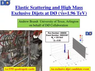
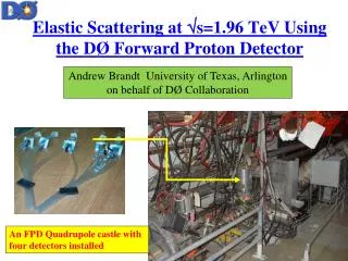
Elastic Scattering at s=1.96 TeV Using the DØ Forward Proton Detector Andrew Brandt University of Texas, Arlington on behalf of DØ Collaboration An FPD Quadrupole castle with four detectors installed
Elastic Scattering • The particles after scattering are the same as the incident particles • =p/p=0 for elastic events; • The cross section can be written as: • This has the same form as light diffracting from a small absorbing disk, hence processes with an intact proton (or two) are called diffractive phenomena • Characterized by a steeply falling |t| distribution and a dip where the slope becomes much flatter Elastic “dip” Structure from Phys. Rev. Lett. 54, 2180 (1985). t = -(pi-pf)2
Forward Proton Detector • There are eight quadrupole spectrometers (Up, Down, In, Out) on the outgoing proton (P) and anti-proton (A) sides each comprised of two detectors (1, 2) • Use Tevatron lattice and scintillating fiber hits to reconstruct and |t| of scattered protons (anti-protons) • The acceptance for |t|>|tmin| where tmin is a function of pot position: • for standard operating conditions |t| > 0.8 GeV2
FPD Detectors • 3 layers in detector: U and V at 45o degrees to X, 90o degrees to each other • Each layer has two planes (prime and unprimed) offset by ~2/3 fiber • Each channel contains four fibers • Two detectors in a spectrometer • Scintillator for timing 17.39 mm V’ V Trigger X’ X U’ U 17.39 mm 1 mm 0.8 mm 3.2 mm
Large β* Store • In 2005 DØ proposed a store with special optics to maximize the |t| acceptance of the FPD • In February 2006, the accelerator was run with the injection tune, β* =1.6m (about 5x larger than normal) • Only 1 proton and 1 anti-proton bunch were injected • Separators OFF (no worries about parasitic collisions with only one bunch) • Integrated Luminosity (30 ± 4 nb-1) was determined by comparing the number of jets from Run IIA measurements with the number in the Large β* store • A total of 20 million events were recorded with a special FPD trigger list
Track Finding • Alignment. • Use over-constrained tracks that pass through horizontal and vertical detectors to do relative alignment of detectors and use hit distributions to align detectors with respect to beam. • Hit Finding • Require less than 5 hit fibers per layer (suppresses beam background) • Use intersection of fiber layers to determine a hit • Track Reconstruction. • Reconstruct the tracks in the forward detectors if there are good hits in both detectors • Use the aligned hit values and the Tevatron lattice transport equations to reconstruct track.
LM A1U A2U Proton P1D P2D Elastic Spectrometer Combinations Anti-proton Elastic events have tracks in diagonally opposite spectrometers Anti-proton Proton Momentum dispersion in horizontal plane results in more halo (beam background) in the IN/OUT detectors, so concentrate on vertical plane AU-PD and AD-PU to maximize |t| acceptance while minimizing background AU-PD combination has the best |t| acceptance
Hit Finding • Combination of fibers in a plane determine a segment • Need two out of three possible segments to get a hit • U/V, U/X, X/V (or U/X/V) • reconstruct x and y position in detecor • use alignment to go from detector to beam coordinates • Can also get an x directly from the x segment (can compare these x measurements to measure resolution) X U V beam
Fiber Correlations within a Detector Correlations between fibers in the primed and unprimed plane of each layer in AU-PD elastic candidates
Layer Multiplicity for Elastic Candidates Elastic events have low fiber multiplicity
Detector Resolutions xuv-xx=2
LM A1U A2U Proton Halo -109 nsec -78 nsec P1D P2D Halo Rejection 78 nsec 109 nsec • The in-time bit is set if a pulse detected in the in-time window • (consistent with a proton originating from the IP) • The halo bit is set if a pulse detected in early time window • (consistent with a halo proton) • We can reject a large fraction of halo events using the timing scintillators (depending on the pot locations)
Correlations Between Detectors fiducial region Elastic Halo
Measuring Cross Section Count elastic events Divide by luminosity Correct for acceptance and efficiency Unsmearing correction for |t| resolution Subtract residual halo background Take weighted average of four measurements (2 elastic configurations each with two pot positions)
“smearing” “true” “observed” “unsmearing” or “unfolding” Correcting Cross Section • Corrections: • f acceptance (geometrical loss due to finite size of opposite spectrometer) • Unsmearing correction due to beam divergence, |t| resolution (standard approach using ansatz function) • Efficiency: use triggers requiring A1-P1 or A2-P2 hits, offline demand 3rd hit, then measure efficiency of 4th detector • Use side bands to measure and subtract background
|t| Resolution ranges from 0.02 at low |t| to 0.045 at high |t| Observe expected colinearity between proton and anti-proton
Measurement of Elastic Slope (b) • Systematic error dominated by trigger • efficiency correction • Second biggest uncertainty (alignment) • = ± 0.3 GeV2 First measurement of b at s=1.96 TeV
d/d|t| Compared to E710+CDF E710/CDF for s=1.8 TeV; GeV2 expect logarithmic dependence with s
d/d|t| Compared to UA4 Slope steeper and slope change earlier for higher s (shrinkage)
Conclusions • We have measured d/d|t| for elastic scattering over the range: 0.2< |t| <1.2 GeV2 the first such measurement at s=1.96 TeV • For 0.2<|t|<0.6 GeV2 we have measured the elastic slope b=16.5 ± 0.1 ± 0.8 GeV-2 • We observe that the elastic slope is steeper and changes slope earlier than lower energy data such as UA4
It’s been a long road from 1999 when the first castle arrived at Fermilab…