Download
1 / 41
410 likes | 436 Views
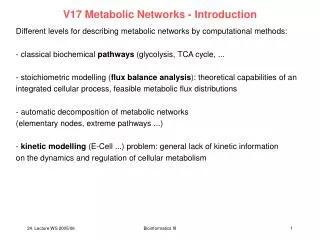
V15 Flux Balance Analysis – Extreme Pathways. Stoichiometric matrix S : m × n matrix with stochiometries of the n reactions as columns and participations of m metabolites as rows. The stochiometric matrix is an important part of the in silico model.

E N D
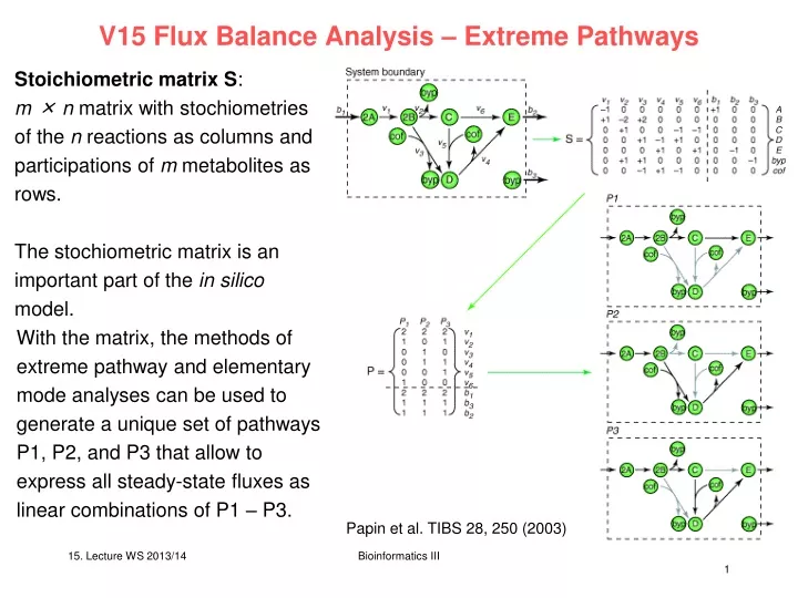
V15 Flux Balance Analysis – Extreme Pathways Stoichiometric matrix S: m × n matrix with stochiometries of the n reactions as columns and participations of m metabolites as rows. The stochiometric matrix is an important part of the in silico model. With the matrix, the methods of extreme pathway and elementary mode analyses can be used to generate a unique set of pathways P1, P2, and P3 that allow to express all steady-state fluxes as linear combinations of P1 – P3. Papin et al. TIBS 28, 250 (2003) Bioinformatics III
Flux balancing Any chemical reaction requiresmass conservation. Therefore one may analyze metabolic systems by requiring mass conservation. Only required: knowledge about stoichiometry of metabolic pathways. For each metabolite Xi : dXi /dt = Vsynthesized – Vused + Vtransported_in – Vtransported_out Bioinformatics III
Flux balancing Under steady-state conditions, the mass balance constraints in a metabolic network can be represented mathematically by the matrix equation: S· v = 0 where the matrix S is the stoichiometric matrix and the vector v represents all fluxes in the metabolic network, including the internal fluxes, transport fluxes and the growth flux. Bioinformatics III
Flux balance analysis Since the number of metabolites is generally smaller than the number of reactions (m < n) the flux-balance equation is typically underdetermined. Therefore there are generally multiple feasible flux distributions that satisfy the mass balance constraints. The set of solutions are confined to the nullspace of matrix S. S . v = 0 Bioinformatics III
Null space: space of feasible solutions Bioinformatics III
Feasible solution set for a metabolic reaction network The steady-state operation of the metabolic network is restricted to the region within a pointed cone, defined as the feasible set. The feasible set contains all flux vectors that satisfy the physicochemical constrains. Thus, the feasible set defines the capabilities of the metabolic network. All feasible metabolic flux distributions lie within the feasible set. Edwards & Palsson PNAS 97, 5528 (2000) Bioinformatics III
True biological flux To find the „true“ biological flux in cells ( e.g. Heinzle, UdS) one needs additional (experimental) information, or one may impose constraints on the magnitude of each individual metabolic flux. The intersection of the nullspace and the region defined by those linear inequalities defines a region in flux space = the feasible set of fluxes. In the limiting case, where all constraints on the metabolic network are known, such as the enzyme kinetics and gene regulation, the feasible set may be reduced to a single point. This single point must lie within the feasible set. Bioinformatics III
E.coli in silico • Best studied cellular system: E. coli. • In 2000, Edwards & Palsson constructed an in silico representation of • E.coli metabolism. • There were 2 good reasons for this: • genome of E.coli MG1655 was already completely sequenced, • Because of long history of E.coli research, biochemical literature, genomic information, metabolic databases EcoCyc, KEGG contained biochemical or genetic evidence for every metabolic reaction included in the in silico representation. In most cases, there existed both. Edwards & Palsson PNAS 97, 5528 (2000) Bioinformatics III
Genes included in in silico model of E.coli Edwards & Palsson PNAS 97, 5528 (2000) Bioinformatics III
E.coli in silico – Flux balance analysis Define i = 0 for irreversible internal fluxes, i = -for reversible internal fluxes (use biochemical literature) Transport fluxes for PO42-, NH3, CO2, SO42-, K+, Na+ were unrestrained. For other metabolites except for those that are able to leave the metabolic network (i.e. acetate, ethanol, lactate, succinate, formate, pyruvate etc.) Find particular metabolic flux distribution in feasible set by linear programming. LP finds a solution that minimizes a particular metabolic objective–Z (subject to the imposed constraints) where e.g. When written in this way, the flux balance analysis (FBA) method finds the solution that maximizes the sum of all fluxes = gives maximal biomass. Edwards & Palsson, PNAS 97, 5528 (2000) Bioinformatics III
E.coli in silico Examine changes in the metabolic capabilities caused by hypothetical gene deletions. To simulate a gene deletion, the flux through the corresponding enzymatic reaction was restricted to zero. Compare optimal value of mutant (Zmutant) to the „wild-type“ objective Z to determine the systemic effect of the gene deletion. Edwards & Palsson PNAS 97, 5528 (2000) Bioinformatics III
Rerouting of metabolic fluxes (Black) Flux distribution for the wild-type. (Red) zwf- mutant. Biomass yield is 99% of wild-type result. (Blue) zwf- pnt- mutant. Biomass yield is 92% of wildtype result. Note how E.coli in silico circumvents removal of one critical reaction (red arrow) by increasing the flux through the alternative G6P P6P reaction. Edwards & Palsson PNAS 97, 5528 (2000) Bioinformatics III
Gene deletions in central intermediary metabolism Maximal biomass yields on glucose for all possible single gene deletions in the central metabolic pathways (gycolysis, pentose phosphate pathway (PPP), TCA, respiration). The results were generated in a simulated aerobic environment with glucose as the carbon source. The transport fluxes were constrained as follows: glucose = 10 mmol/g-dry weight (DW) per h; oxygen = 15 mmol/g-DW per h. The maximal yields were calculated by using FBA with the objective of maximizing growth. Yellow bars: gene deletions that reduced the maximal biomass yield of Zmutant to less than 95% of the in silico wild type Zwt. Edwards & Palsson PNAS 97, 5528 (2000) Bioinformatics III
Interpretation of gene deletion results The essential gene products were involved in the 3-carbon stage of glycolysis, 3 reactions of the TCA cycle, and several points within the pentose phosphate pathway (PPP). The remainder of the central metabolic genes could be removed while E.coli in silico maintained the potential to support cellular growth. This suggests that a large number of the central metabolic genes can be removed without eliminating the capability of the metabolic network to support growth under the conditions considered. Edwards & Palsson PNAS 97, 5528 (2000) Bioinformatics III
E.coli in silico – validation + and – means growth or no growth. means that suppressor mutations have been observed that allow the mutant strain to grow. 4 virtual growth media: glc: glucose, gl: glycerol, succ: succinate, ac: acetate. In 68 of 79 cases, the prediction was consistent with exp. predictions. Red and yellow circles: predicted mutants that eliminate or reduce growth. Edwards & Palsson PNAS 97, 5528 (2000) Bioinformatics III
Summary - FBA FBA analysis constructs the optimal network utilization simply using the stoichiometry of metabolic reactions and capacity constraints. For E.coli the in silico results are mostly consistent with experimental data. FBA shows that the E.coli metabolic network contains relatively few critical gene products in central metabolism. However, the ability to adjust to different environments (growth conditions) may be diminished by gene deletions. FBA identifies „the best“ the cell can do, not how the cell actually behaves under a given set of conditions. Here, survival was equated with growth. FBA does not directly consider regulation or regulatory constraints on the metabolic network. This can be treated separately (see future lecture). Edwards & Palsson PNAS 97, 5528 (2000) Bioinformatics III
Idea – extreme pathways A torch is directed at an open door and shines into a dark room ... What area is lighted ? Instead of marking all lighted points individually, it would be sufficient to characterize the „extreme rays“ that go through the corners of the door. The lighted area is the area between the extreme rays = linear combinations of the extreme rays. Bioinformatics III
Extreme Pathways introduced into metabolic analysis by the lab of Bernard Palsson (Dept. of Bioengineering, UC San Diego). The publications of this lab are available at http://gcrg.ucsd.edu/publications/index.html The extreme pathway technique is based on the stoichiometric matrix representation of metabolic networks. All external fluxes are defined as pointing outwards. Schilling, Letscher, Palsson, J. theor. Biol. 203, 229 (2000) Bioinformatics III
Idea – extreme pathways S Shaded area: x ≥ 0 Shaded area: x1 ≥ 0 ∧x2 ≥ 0 Either S.x ≥ 0 (S acts as rotation matrix) or find optimal vectors change coordinate system from x1, x2to r1, r2. Duality of two matrices S and R. Shaded area: r1 ≥ 0 ∧r2 ≥ 0 Edwards & Palsson PNAS 97, 5528 (2000) Bioinformatics III
Extreme Pathways – algorithm - setup The algorithm to determine the set of extreme pathways for a reaction network follows the pinciples of algorithms for finding the extremal rays/ generating vectors of convex polyhedral cones. Combine n n identity matrix (I) with the transpose of the stoichiometric matrix ST. I serves for bookkeeping. Schilling, Letscher, Palsson, J. theor. Biol. 203, 229 (2000) S I ST Bioinformatics III
separate internal and external fluxes Examine constraints on each of the exchange fluxes as given by j bj j If the exchange flux is constrained to be positive do nothing. If the exchange flux is constrained to be negative multiply the corresponding row of the initial matrix by -1. If the exchange flux is unconstrained move the entire row to a temporary matrix T(E). This completes the first tableau T(0). T(0) and T(E) for the example reaction system are shown on the previous slide. Each element of these matrices will be designated Tij. Starting with i = 1 and T(0) = T(i-1) the next tableau is generated in the following way: Schilling, Letscher, Palsson, J. theor. Biol. 203, 229 (2000) Bioinformatics III
idea of algorithm (1) Identify all metabolites that do not have an unconstrained exchange flux associated with them. The total number of such metabolites is denoted by . The example system contains only one such metabolite, namely C ( = 1). What is the main idea? - We want to find balanced extreme pathways that don‘t change the concentrations of metabolites when flux flows through (input fluxes are channelled to products not to accumulation of intermediates). - The stochiometrix matrix describes the coupling of each reaction to the concentration of metabolites X. - Now we need to balance combinations of reactions that leave concentrations unchanged. Pathways applied to metabolites should not change their concentrations the matrix entries need to be brought to 0. Schilling, Letscher, Palsson, J. theor. Biol. 203, 229 (2000) Bioinformatics III
keep pathways that do not change concentrations of internal metabolites (2) Begin forming the new matrix T(i) by copying all rows from T(i – 1) which already contain a zero in the column of ST that corresponds to the first metabolite identified in step 1, denoted by index C. (Here 3rd column of ST.) Schilling, Letscher, Palsson, J. theor. Biol. 203, 229 (2000) A B C D E T(0) = T(1) = + Bioinformatics III
balance combinations of other pathways (3) Of the remaining rows in T(i-1) add together all possible combinations of rows which contain values of the opposite sign in column C, such that the addition produces a zero in this column. Schilling, et al. JTB 203, 229 T(0) = T(1) = 1 2 3 4 5 6 7 8 9 10 11 Bioinformatics III
remove “non-orthogonal” pathways (4) For all rows added to T(i) in steps 2 and 3 check that no row exists that is a non-negative combination of any other rows in T(i) . One method for this works as follows: let A(i) = set of column indices j for which the elements of row i = 0. For the example above Then check to determine if there exists A(1) = {2,3,4,5,6,9,10,11} another row (h) for which A(i) is a A(2) = {1,4,5,6,7,8,9,10,11} subset of A(h). A(3) = {1,3,5,6,7,9,11} A(4) = {1,3,4,5,7,9,10} If A(i) A(h),i h A(5) = {1,2,4,6,7,9,11} where A(6) = {1,2,3,6,7,8,9,10,11} A(i) = { j : Ti,j = 0, 1 j (n+m) } A(7) = {1,2,3,4,7,8,9} then row i must be eliminated from T(i) Schilling et al. JTB 203, 229 Bioinformatics III
repeat steps for all internal metabolites (5) With the formation of T(i) complete steps 2 – 4 for all of the metabolites that do not have an unconstrained exchange flux operating on the metabolite, incrementing i by one up to . The final tableau will be T(). Note that the number of rows in T() will be equal to k, the number of extreme pathways. Schilling et al. JTB 203, 229 Bioinformatics III
balance external fluxes (6) Next we append T(E) to the bottom of T(). (In the example here = 1.) This results in the following tableau: Schilling et al. JTB 203, 229 T(1/E) = Bioinformatics III
balance external fluxes (7) Starting in the n+1 column (or the first non-zero column on the right side), if Ti,(n+1) 0 then add the corresponding non-zero row from T(E) to row i so as to produce 0 in the n+1-th column. This is done by simply multiplying the corresponding row in T(E) by Ti,(n+1) and adding this row to row i . Repeat this procedure for each of the rows in the upper portion of the tableau so as to create zeros in the entire upper portion of the (n+1) column. When finished, remove the row in T(E) corresponding to the exchange flux for the metabolite just balanced. Schilling et al. JTB 203, 229 Bioinformatics III
balance external fluxes (8) Follow the same procedure as in step (7) for each of the columns on the right side of the tableau containing non-zero entries. (In our example we need to perform step (7) for every column except the middle column of the right side which correponds to metabolite C.) The final tableau T(final) will contain the transpose of the matrix P containing the extreme pathways in place of the original identity matrix. Schilling et al. JTB 203, 229 Bioinformatics III
pathway matrix T(final) = PT = Schilling et al. JTB 203, 229 v1 v2 v3 v4 v5 v6 b1 b2 b3 b4 p1 p7 p3 p2 p4 p6 p5 Bioinformatics III
Extreme Pathways for model system 2 pathways p6 and p7 are not shown in the bottom fig. because all exchange fluxes with the exterior are 0. Such pathways have no net overall effect on the functional capabilities of the network. They belong to the cycling of reactions v4/v5 and v2/v3. Schilling et al. JTB 203, 229 v1 v2 v3 v4 v5 v6 b1 b2 b3 b4 p1 p7 p3 p2 p4 p6 p5 Bioinformatics III
How reactions appear in pathway matrix In the matrix P of extreme pathways, each column is an EP and each row corresponds to a reaction in the network. The numerical value of the i,j-th element corresponds to the relative flux level through the i-th reaction in the j-th EP. Papin, Price, Palsson, Genome Res. 12, 1889 (2002) Bioinformatics III 15. Lecture WS 2012/13
Properties of pathway matrix After normalizing P to a matrix with entries 0 or 1, the symmetric Pathway Length Matrix PLM can be calculated: where the values along the diagonal correspond to the length of the EPs. The off-diagonal terms of PLM are the number of reactions that a pair of extreme pathways have in common. Papin, Price, Palsson, Genome Res. 12, 1889 (2002) Bioinformatics III 15. Lecture WS 2012/13
Properties of pathway matrix One can also compute a reaction participation matrix PPM from P: where the diagonal correspond to the number of pathways in which the given reaction participates. Papin, Price, Palsson, Genome Res. 12, 1889 (2002) Bioinformatics III 15. Lecture WS 2012/13
EP Analysis of H. pylori and H. influenza Amino acid synthesis in Heliobacter pylori vs. Heliobacter influenza studied by EP analysis. Papin, Price, Palsson, Genome Res. 12, 1889 (2002) Bioinformatics III
Extreme Pathway Analysis Calculation of EPs for increasingly large networks is computationally intensive and results in the generation of large data sets. Even for integrated genome-scale models for microbes under simple conditions, EP analysis can generate thousands or even millions of vectors! It turned out that the number of reactions that participate in EPs that produce a particular product is usually poorly correlated to the product yield and the molecular complexity of the product. Possible way out? Matrix diagonalisation – eigenvectors: only possible for quadratic n × n matrices with rank n. Papin, Price, Palsson, Genome Res. 12, 1889 (2002) Bioinformatics III
Quasi-diagonalisation of pathway matrix by SVD Suppose M is an m n matrix with real or complex entries. Then there exists a factorization of the form M = U V* where U : m m unitary matrix, (U*U = UU* = I) Σ : is an mn matrix with nonnegative numbers on the diagonal and zeros off the diagonal, V* : the transpose of V, is an n n unitary matrix of real or complex numbers. Such a factorization is called a singular-value decomposition of M. U describes the rows of M with respect to the base vectors associated with the singular values. V describes the columns of M with respect to the base vectors associated with the singular values. Σ contains the singular values. One commonly insists that the values Σi,i be ordered in non-increasing fashion. Then, the diagonal matrix Σ is uniquely determined by M (but not U and V). Bioinformatics III
Single Value Decomposition of EP matrices For a given EP matrix P np, SVD decomposes Pinto 3 matrices where U nn : orthonormal matrix of the left singular vectors, Vpp : an analogous orthonormal matrix of the right singular vectors, rr :a diagonal matrix containing the singular values i=1..rarranged in descending order where r is the rank of P. The first r columns of U and V, referred to as the left and right singular vectors, or modes, are unique and form the orthonormal basis for the column space and row space of P. The singular values are the square roots of the eigenvalues of PTP. The magnitudes of the singular values in indicate the relative contribution of the singular vectors in U and V in reconstructing P. E.g. the second singular value contributes less to the construction of P than the first singular value etc. Price et al. Biophys J 84, 794 (2003) Bioinformatics III
Single Value Decomposition of EP: Interpretation The first mode (as the other modes) corresponds to a valid biochemical pathway through the network. The first mode will point into the portions of the cone with highest density of EPs. Price et al. Biophys J 84, 794 (2003) Bioinformatics III
SVD applied for Heliobacter systems Cumulative fractional contributions for the SVD of the EP matrices of H. influenza and H. pylori. This plot represents the contribution of the first n modes to the overall description of the system. Ca. 20 modes allow describing most of the metabolic activity in the Network. Cumulative fractional contribution : sum of the first n fractional singular values. This value represents the contribution of the first n modes to the overall description of the system. The rank of the respective extreme pathway matrix is shown for nonessential amino acids. Scrit: number of singular values that account for 95% of the variance in the matrices. Entries with ‘‘- - -’’ correspond to essential amino acids. Price et al. Biophys J 84, 794 (2003) Bioinformatics III
Summary – Extreme Pathways Extreme Pathway Analysis is a standard technique for analysis of metabolic networks. Number of EPs can become extremely large – hard to interpret. EP is an excellent basis for studying systematic effects of reaction cut sets. SVD could facilitate analysis of EPs. Has not been widely used sofar. It will be very important to consider the interplay of metabolic and regulatory networks. Bioinformatics III