Download

1 / 10
100 likes | 207 Views
Analysis Using R. 1.Finds the classical scaling solution. 2. Computes the Trace criterion & Magnitude criterion to determine the # of dimensions. (1*). R>voles_mds<- cmdscale(watervoles, k=13, eig=TRUE). R>voles_mds$eig

E N D
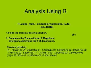
Analysis Using R 1.Finds the classical scaling solution. 2. Computes the Trace criterion & Magnitude criterion to determine the # of dimensions. (1*) R>voles_mds<- cmdscale(watervoles, k=13, eig=TRUE) R>voles_mds$eig [1] 7.359910e-01 2.626003e-01 1.492622e-01 6.990457e-02 2.956972e-02 1.931184e-02 8.326673e-17 -1.139451e-02 -1.279569e-02 -2.849924e-02 [11] -4.251502e-02 -5.255450e-02 -7.406143e-02
We have 13 eigenvalues, some positive & some negative. R>sum(abs(voles_mds$eig[1:2]))/ sum (abs(voles_mds$eig)) [1] 0.6708889 This code satisfies Magnitude Criterion. (2*) R>sum((voles_mds$eig[1:2])^2/ sum((voles_mds$eig)^2) [1] 0.9391378 Which is the criteria suggested by Mardia et al.; the above code is exactly: k n ∑│λ│ / ∑ │λ│ i=1 i=1 0.6708889 & .9391378 are large enough to suggest that the original distances Between water vole populations can be represented adequately in two dimensions. (3*)
R>x<- voles_mds$points[, 1] 1: Coordinate 1 R>y<-voles_mds$points[, 2] 2: Coordinate 2 R>plot(x,y,xlab= "Coordinate 1", ylab= "Coordinate 2", xlim= range(x) * 1.2, type= "n") R>text(x,y, labels= colnames(watervoles)) 6 British populations are close to populations living in the Alps, Yugoslavia, Germany, Norway, & Pyrenees I. (Arvicola terrestris) These British populations are distant from the populations in Pyrenees II, North Spain and South Spain. (Arvicola sapidus) (4*)
Minimum Spanning Tree (MDS solution) highlight possible distortions. (5,6*) Links of a minimum spanning tree of the proximity matrix may be plotted onto the two-dimensional scaling representation to identify distortions (if any) produced by scaling solutions. These distortions look like nearby points on the plot that are not linked by an edge of a tree. (7*) R>library("ape") R>st<- mst(watervoles) R>plot(x,y,xlab= "Coordinate 1", ylab= "Coordinate 2", xlim= range (x) * 1.2, type= "n") R>for (i in 1:nrow(watervoles)) { + w1<- which(st[i, ] == 1) + segments(x[i], y[i], x[w1], y[w1]) } R>text(x, y, labels= colnames(watervoles))
The apparent closeness of the populations, Germany & Norway, by the points suggested here in this MDS solution, does not reflect accurately their calculated dissimilarity. (8*)
Non-Metric Scaling Example: Analyzing Voting Behavior among Republicans. R Function isoMDS from package “MASS” R>library("MASS") R>data("voting", package= "HSAUR") R>voting_mds<- isoMDS(voting)
Two-Dimensional Solution: R>x<- voting_mds$points[, 1] R>y<- voting_mds$points[, 2] R>plot(x,y, xlab="Coordinate 1", ylab= "Coordinate 2", + xlim= range(voting_mds$points[, 1]) *1.2, + type= "n" ) R>text(x,y, labels= colnames(voting)) R>voting_sh<- Shepard(voting[ lower.tri(voting)], + voting_mds$points Figure suggests that there is more variation in voting behavior among Republicans. (*9)
R>library("MASS") R>voting_sh<- Shepard(voting[lower.tri(voting)], + voting_mds$points) R>plot(voting_sh, pc= ".", xlab= "Dissimilarity", + ylab= "Distance", xlim= range(voting_sh$x), + ylim= range(voting_sh$x)) R>lines(voting_sh$x, voting_sh$yf, type= "S") Quality of a multidimensional scaling can be assessed informally by plotting the original dissimilarities & the distances obtained from a multidimensional scaling in a scatterplot. Ideally, all the lines should fall on the bisecting line.