Download
1 / 52
530 likes | 652 Views
Part 2 Roots of Equations. Why? But. All Iterative. Chapter 5 Bracketing Methods (Or, two point methods for finding roots). Two initial guesses for the root are required. These guesses must “bracket” or be on either side of the root. == > Fig. 5.1

E N D
Part 2 Roots of Equations Why? But
Chapter 5Bracketing Methods(Or, two point methods for finding roots) • Two initial guesses for the root are required. These guesses must “bracket” or be on either side of the root. == > Fig. 5.1 • If one root of a real and continuous function, f(x)=0, is bounded by values x=xl, x=xu then f(xl) . f(xu) <0. (The function changes sign on opposite sides of the root)
The Bisection Method For the arbitrary equation of one variable, f(x)=0 • Pick xl and xu such that they bound the root of interest, check if f(xl).f(xu) <0. • Estimate the root by evaluating f[(xl+xu)/2]. • Find the pair • If f(xl). f[(xl+xu)/2]<0, root lies in the lower interval, then xu=(xl+xu)/2 and go to step 2.
If f(xl). f[(xl+xu)/2]>0, root lies in the upper interval, then xl= [(xl+xu)/2, go to step 2. • If f(xl). f[(xl+xu)/2]=0, then root is (xl+xu)/2 and terminate. • Compare es with ea (5.2, p. 118) • If ea<es, stop. Otherwise repeat the process.
Pros Easy Always find root Number of iterations required to attain an absolute error can be computed a priori. Cons Slow Know a and b that bound root Multiple roots No account is taken of f(xl) and f(xu), if f(xl) is closer to zero, it is likely that root is closer to xl . Evaluation of Method
How Many Iterations will It Take? • Length of the first Interval Lo=b-a • After 1 iteration L1=Lo/2 • After 2 iterations L2=Lo/4 • After k iterations Lk=Lo/2k
If the absolute magnitude of the error is and Lo=2, how many iterations will you have to do to get the required accuracy = 10-4 in the solution?
The False-Position Method(Regula-Falsi) • If a real root is bounded by xl and xu of f(x)=0, then we can approximate the solution by doing a linear interpolation between the points [xl, f(xl)] and [xu, f(xu)] to find the xr value such that l(xr)=0, l(x) is the linear approximation of f(x). == > Fig. 5.12
Procedure • Find a pair of values of x, xl and xu such that fl=f(xl) <0 and fu=f(xu) >0. • Estimate the value of the root from the following formula (Refer to Box 5.1) and evaluate f(xr).
Use the new point to replace one of the original points, keeping the two points on opposite sides of the x axis. Use the same selecting rules as the bisection method. If f(xr)=0 then you have found the root and need go no further.
See if the new xl and xu are close enough for convergence to be declared. If they are not go back to step 2. • Why this method? • Usually faster • Always converges for a single root. See Sec.5.3.1, Pitfalls of the False-Position Method Note: Always check by substituting estimated root in the original equation to determine whether f(xr) ≈ 0. • One-sidedness: Watch out (p. 128)
Chapter 6Open Methods Figure 6.1 • Open methods are based on formulas that require only a single starting value of x or two starting values that do not necessarily bracket the root.
Simple Fixed-point Iteration • Rearrange the function so that x is on the left side of the equation: • Bracketing methods are “convergent”. • Fixed-point methods may sometime “diverge”, depending on the stating point (initial guess) and how the function behaves. • Good for calculators.
Convergence Figure 6.2 • x=g(x) can be expressed as a pair of equations: y1=x y2=g(x) (component equations) • Plot them separately.
Conclusion • Fixed-point iteration converges if • When the method converges, the error is roughly proportional to or less than the error of the previous step, therefore it is called “linearly convergent.”
Newton-Raphson Method • Most widely used method. • Based on Taylor series expansion: Solve for Newton-Raphson formula
Fig. 6.5 • A convenient method for functions whose derivatives can be evaluated analytically. It may not be convenient for functions whose derivatives cannot be evaluated analytically.
The Secant Method • A slight variation of Newton’s method for functions whose derivatives are difficult to evaluate. For these cases the derivative can be approximated by a backward finite divided difference.
Fig. 6.7 • Requires two initial estimates of x , e.g, xo, x1. However, because f(x) is not required to change signs between estimates, it is not classified as a “bracketing” method. • The scant method has the same properties as Newton’s method. Convergence is not guaranteed for all xo, f(x).
Multiple Roots • None of the methods deal with multiple roots efficiently, however, one way to deal with problems is as follows: This function has roots at all the same locations as the original function
“Multiple root” corresponds to a point where a function is tangent to the x axis. • Difficulties • Function does not change sign at the multiple root, therefore, cannot use bracketing methods. • Both f(x) and f′(x)=0, division by zero with Newton’s and Secant methods.
Taylor series expansion of a function of more than one variable • The root of the equation occurs at the value of x and y where ui+1 and vi+1 equal to zero.
A set of two linear equations with two unknowns that can be solved for.
Chapter 7Roots of Polynomials • The roots of polynomials such as • Follow these rules: • For an nth order equation, there are n real or complex roots. • If n is odd, there is at least one real root. • If complex root exist in conjugate pairs (that is, l+mi and l-mi), where i=sqrt(-1).
Conventional Methods • The efficacy of bracketing and open methods depends on whether the problem being solved involves complex roots. If only real roots exist, these methods could be used. However, • Finding good initial guesses complicates both the open and bracketing methods, also the open methods could be susceptible to divergence. • Special methods have been developed to find the real and complex roots of polynomials – Müller and Bairstow methods.
Müller Method • Müller’s method obtains a root estimate by projecting a parabola to the x axis through three function values. Figure 7.3
Müller Method • The method consists of deriving the coefficients of parabola that goes through the three points: • 1. Write the equation in a convenient form:
The parabola should intersect the three points [xo, f(xo)], [x1, f(x1)], [x2, f(x2)]. The coefficients of the polynomial can be estimated by substituting three points to give • Three equations can be solved for three unknowns, a, b, c. Since two of the terms in the 3rd equation are zero, it can be immediately solved for c=f(x2).
Roots can be found by applying an alternative form of quadratic formula: • The error can be calculated as • ±term yields two roots, the sign is chosen to agree with b. This will result in a largest denominator, and will give root estimate that is closest to x2.
Once x3 is determined, the process is repeated using the following guidelines: • If only real roots are being located, choose the two original points that are nearest the new root estimate, x3. • If both real and complex roots are estimated, employ a sequential approach just like in secant method, x1, x2, and x3 to replace xo, x1, and x2.
Bairstow’s Method • Bairstow’s method is an iterative approach loosely related to both Müller and Newton Raphson methods. • It is based on dividing a polynomial by a factor x-t:
To permit the evaluation of complex roots, Bairstow’s method divides the polynomial by a quadratic factor x2-rx-s:
For the remainder to be zero, boand b1 must be zero. However, it is unlikely that our initial guesses at the values of r and s will lead to this result, a systematic approach can be used to modify our guesses so that boand b1 approach to zero. • Using a similar approach to Newton Raphson method, both bo and b1can be expanded as function of both r and s in Taylor series.
If partial derivatives of the b’s can be determined, then the two equations can be solved simultaneously for the two unknowns Dr and Db. • Partial derivatives can be obtained by a synthetic division of the b’s in a similar fashion the b’s themselves are derived: