Download
1 / 20
200 likes | 313 Views
Adding Totals Data Labels to an Excel 2007 Stacked Bar Chart. Robert Rosen. In an Excel 2007 stacked bar graph, you can use the <add data labels> feature to show the numeric values of each component in the stack, like this….

E N D
Adding Totals Data Labels to an Excel 2007 Stacked Bar Chart Robert Rosen
In an Excel 2007 stacked bar graph, you can use the <add data labels> feature to show the numeric values of each component in the stack, like this…
…but what if you want to show the total value of the entire stack, like this? Excel doesn’t have a “show totals” option • Answer: use a Trick!
Step 1: Add Data Labels Click on the border of the chart to select it, then Chart ToolsLayoutData Labels (in this example, we select “Center”) Dots show when chart is selected
Step 2: Add a totals column to the source data (if not already existant)
Step 3: Add a new data series to the chart for the totals Right-click in the chart to bring up this menu, then click “Select Data”
Step 4: Change the totals series to a line graph Select the Total series and right-click to bring up this menu, then click “Change Series Chart Type”
Step 4 (contd.) Select a Line graph
Step 5: Move the labels to above the series Select a label and right-click to bring up this menu, then “Format Data Labels”
Step 5 (contd.) Select “Label Options”, then for Label Position, “Above”
Step 6: Hide the line Select the line and right-click to bring up this menu, then “Format Data Series”
Step 6 (contd) Select “Line Color”, then “No line”
Step 7: Delete the legend entry Select the Totals legend text and right-click to bring up this menu, then “Delete”