Download
1 / 27
280 likes | 456 Views
Query Optimization. Goal:. Declarative SQL query. Imperative query execution plan:. buyer. SELECT S.buyer FROM Purchase P, Person Q WHERE P.buyer=Q.name AND Q.city=‘seattle’ AND Q.phone > ‘5430000’ . . City=‘seattle’. phone>’5430000’. Inputs: the query

E N D
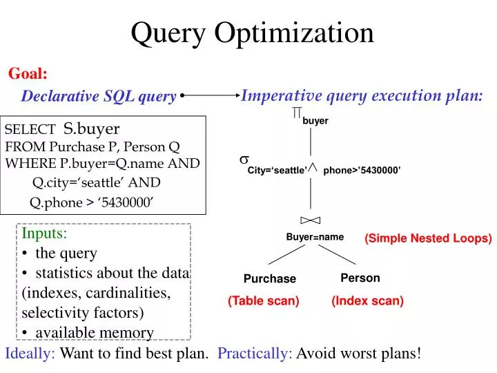
Query Optimization Goal: Declarative SQL query Imperative query execution plan: buyer SELECT S.buyer FROM Purchase P, Person Q WHERE P.buyer=Q.name AND Q.city=‘seattle’ AND Q.phone > ‘5430000’ City=‘seattle’ phone>’5430000’ • Inputs: • the query • statistics about the data (indexes, cardinalities, selectivity factors) • available memory Buyer=name (Simple Nested Loops) Person Purchase (Table scan) (Index scan) Ideally: Want to find best plan. Practically: Avoid worst plans!
How are we going to build one? • What kind of optimizations can we do? • What are the issues? • How would we architect a query optimizer?
sname rating > 5 bid=100 sid=sid Sailors Reserves (On-the-fly) sname (On-the-fly) rating > 5 bid=100 (Simple Nested Loops) sid=sid Sailors Reserves RA Tree: Motivating Example SELECT S.sname FROM Reserves R, Sailors S WHERE R.sid=S.sid AND R.bid=100 AND S.rating>5 • Cost: 500+500*1000 I/Os • By no means the worst plan! • Misses several opportunities: selections could have been `pushed’ earlier, no use is made of any available indexes, etc. • Goal of optimization: To find more efficient plans that compute the same answer. Plan:
Schema for Examples Sailors (sid: integer, sname: string, rating: integer, age: real) Reserves (sid: integer, bid: integer, day: dates, rname: string) • Reserves: • Each tuple is 40 bytes long, 100 tuples per page, 1000 pages. • Sailors: • Each tuple is 50 bytes long, 80 tuples per page, 500 pages.
(On-the-fly) sname (Sort-Merge Join) sid=sid (Scan; (Scan; write to write to rating > 5 bid=100 temp T2) temp T1) Reserves Sailors Alternative Plans 1 • Main difference: push selects. • With 5 buffers, cost of plan: • Scan Reserves (1000) + write temp T1 (10 pages, if we have 100 boats, uniform distribution). • Scan Sailors (500) + write temp T2 (250 pages, if we have 10 ratings). • Sort T1 (2*2*10), sort T2 (2*3*250), merge (10+250), total=1800 • Total: 3560 page I/Os. • If we used BNL join, join cost = 10+4*250, total cost = 2770. • If we `push’ projections, T1 has only sid, T2 only sid and sname: • T1 fits in 3 pages, cost of BNL drops to under 250 pages, total < 2000.
(On-the-fly) sname Alternative Plans 2With Indexes (On-the-fly) rating > 5 (Index Nested Loops, with pipelining ) sid=sid • With clustered index on bid of Reserves, we get 100,000/100 = 1000 tuples on 1000/100 = 10 pages. • INL with pipelining (outer is not materialized). (Use hash Sailors bid=100 index; do not write result to temp) Reserves • Join column sid is a key for Sailors. • At most one matching tuple, unclustered index on sid OK. • Decision not to push rating>5 before the join is based on • availability of sid index on Sailors. • Cost: Selection of Reserves tuples (10 I/Os); for each, • must get matching Sailors tuple (1000*1.2); total 1210 I/Os.
Building Blocks • Algebraic transformations (many and wacky). • Statistical model: estimating costs and sizes. • Finding the best join trees: • Bottom-up (dynamic programming): System-R • Newer architectures: • Starburst: rewrite and then tree find • Volcano: all at once, top-down.
Query Optimization Process(simplified a bit) • Parse the SQL query into a logical tree: • identify distinct blocks (corresponding to nested sub-queries or views). • Query rewrite phase: • apply algebraic transformations to yield a cheaper plan. • Merge blocks and move predicates between blocks. • Optimize each block: join ordering. • Complete the optimization: select scheduling (pipelining strategy).
Key Lessons in Optimization • There are many approaches and many details to consider in query optimization • Classic search/optimization problem! • Not completely solved yet! • Main points to take away are: • Algebraic rules and their use in transformations of queries. • Deciding on join ordering: System-R style (Selinger style) optimization. • Estimating cost of plans and sizes of intermediate results.
Operations (revisited) • Scan ([index], table, predicate): • Either index scan or table scan. • Try to push down sargable predicates. • Selection (filter) • Projection (always need to go to the data?) • Joins: nested loop (indexed), sort-merge, hash, outer join. • Grouping and aggregation (usually the last).
Relational Algebra Equivalences • Allow us to choose different join orders and to ‘push’ selections and projections ahead of joins. • Selections: (Cascade) (Commute) (Cascade) • Projections: (Associative) • Joins: R (S T) (R S) T (Commute) (R S) (S R) R (S T) (T R) S • Show that:
More Equivalences • A projection commutes with a selection that only uses attributes retained by the projection. • A selection on just attributes of R commutes with join R S. (i.e., (R S) (R) S ) • Similarly, if a projection follows a join R S, we can ‘push’ it by retaining only attributes of R (and S) that are needed for the join or are kept by the projection.
Query Rewrites: Sub-queries SELECT Emp.Name FROM Emp WHERE Emp.Age < 30 AND Emp.Dept# IN (SELECT Dept.Dept# FROM Dept WHERE Dept.Loc = “Seattle” AND Emp.Emp#=Dept.Mgr)
The Un-Nested Query SELECT Emp.Name FROM Emp, Dept WHERE Emp.Age < 30 AND Emp.Dept#=Dept.Dept# AND Dept.Loc = “Seattle” AND Emp.Emp#=Dept.Mgr
Semi-Joins, Magic Sets • You can’t always un-nest sub-queries (it’s tricky). • But you can often use a semi-join to reduce the computation cost of the inner query. • A magic set is a superset of the possible bindings in the result of the sub-query. • Also called “sideways information passing”. • Great idea; reinvented every few years on a regular basis.
Rewrites: Magic Sets Create View DepAvgSal AS (Select E.did, Avg(E.sal) as avgsal From Emp E Group By E.did) Select E.eid, E.sal From Emp E, Dept D, DepAvgSal V Where E.did=D.did AND D.did=V.did And E.age < 30 and D.budget > 100k And E.sal > V.avgsal
Rewrites: SIPs Select E.eid, E.sal From Emp E, Dept D, DepAvgSal V Where E.did=D.did AND D.did=V.did And E.age < 30 and D.budget > 100k And E.sal > V.avgsal • DepAvgsal needs to be evaluated only for cases where V.did IN Select E.did From Emp E, Dept D Where E.did=D.did And E.age < 30 and D.budget > 100K
So… Supporting Views: 1. Create View ED as (Select E.did From Emp E, Dept D Where E.did=D.did And E.age < 30 and D.budget > 100K) • Create View LAvgSal as (Select E.did Avg(E.Sal) as avgSal From Emp E, ED Where E.did=ED.did Group By E.did)
And Finally… Transformed query: Select ED.eid, ED.sal From ED, Lavgsal Where E.did=ED.did And ED.sal > Lavgsal.avgsal
Rewrites: GroupBy and Join • Schema: • Product (pid, unitprice,…) • Sales(tid, date, store, pid, units) • Trees: Join groupBy(pid) Sum(units) groupBy(pid) Sum(units) Join Products Filter (in NW) Products Filter (in NW) Scan(Sales) Filter(date=Q2,2000) Scan(Sales) Filter(date=Q2,2000)
Rewrites:Operation Introduction groupBy(cid) Sum(amount) • Schema: • Category (pid, cid, details) • Sales(tid, date, store, pid,amount) • Trees: Join groupBy(cid) Sum(amount) groupBy(pid) Sum(amount) Join Category Filter (…) Category Filter (…) Scan(Sales) Filter(store IN {CA,WA}) Scan(Sales) Filter(store IN {CA,WA})
sname sid=sid (Scan; (Scan; write to write to rating > 5 bid=100 temp T2) temp T1) Reserves Sailors sname rating > 5 bid=100 sid=sid Sailors Reserves Query Rewriting: Predicate Pushdown The earlier we process selections, less tuples we need to manipulate higher up in the tree. Disadvantages?
Query Rewrites: Predicate Pushdown (through grouping) Select bid, Max(age) From Reserves R, Sailors S Where R.sid=S.sid GroupBy bid Having Max(age) > 40 Select bid, Max(age) From Reserves R, Sailors S Where R.sid=S.sid and S.age > 40 GroupBy bid Having Max(age) > 40 • For each boat, find the maximal age of sailors who’ve reserved it. • Advantage: the size of the join will be smaller. • Requires transformation rules specific to the grouping/aggregation • operators. • Won’t work if we replace Max by Min.
Query Rewrite:Pushing predicates up Sailing wizz dates: when did the youngest of each sailor level rent boats? Select sid, date From V1, V2 Where V1.rating = V2.rating and V1.age = V2.age Create View V1 AS Select rating, Min(age) From Sailors S Where S.age < 20 GroupBy rating Create View V2 AS Select sid, rating, age, date From Sailors S, Reserves R Where R.sid=S.sid
Query Rewrite: Predicate Movearound Sailing wizz dates: when did the youngest of each sailor level rent boats? Select sid, date From V1, V2 Where V1.rating = V2.rating and V1.age = V2.age, age < 20 First, move predicates up the tree. Create View V1 AS Select rating, Min(age) From Sailors S Where S.age < 20 GroupBy rating Create View V2 AS Select sid, rating, age, date From Sailors S, Reserves R Where R.sid=S.sid
Query Rewrite: Predicate Movearound Sailing wizz dates: when did the youngest of each sailor level rent boats? Select sid, date From V1, V2 Where V1.rating = V2.rating and V1.age = V2.age, andage < 20 First, move predicates up the tree. Then, move them down. Create View V1 AS Select rating, Min(age) From Sailors S Where S.age < 20 GroupBy rating Create View V2 AS Select sid, rating, age, date From Sailors S, Reserves R Where R.sid=S.sid, and S.age < 20.
Query Rewrite Summary • The optimizer can use any semantically correct rule to transform one query to another. • Rules try to: • move constraints between blocks (because each will be optimized separately) • Unnest blocks • Especially important in decision support applications where queries are very complex. • In a few minutes of thought, you’ll come up with your own rewrite. Some query, somewhere, will benefit from it. • Theorems?