Download
1 / 36
370 likes | 492 Views
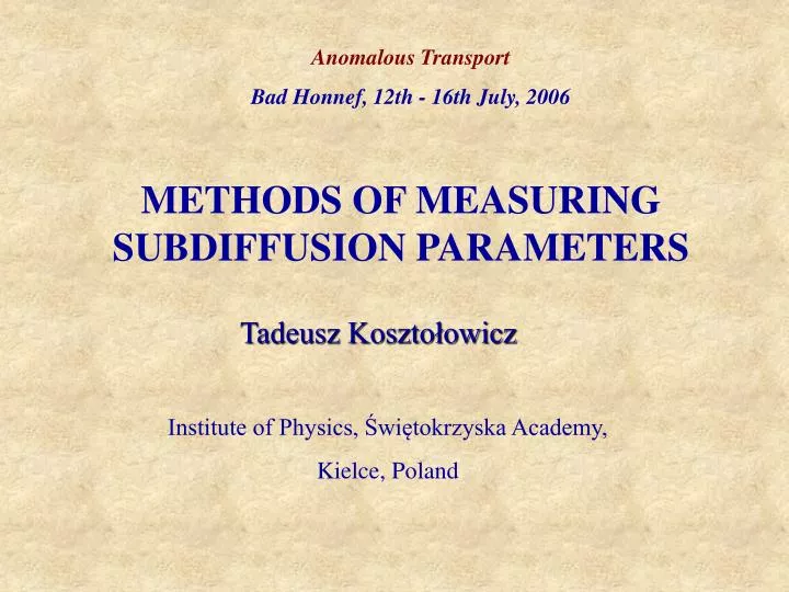
Anomalous Transport Bad Honnef, 12th - 16th July, 2006. METHODS OF MEASURING SUBDIFFUSION PARAMETERS. Tadeusz Kosztołowicz. Institute of Physics, Świętokrzyska Academy, Kielce, Poland. T. Kosztołowicz, Measuring subdiffusion parameters. Introduction. Measuring subdiffusion parameters:

E N D
Anomalous Transport Bad Honnef, 12th - 16th July, 2006 METHODS OF MEASURING SUBDIFFUSION PARAMETERS Tadeusz Kosztołowicz Institute of Physics, Świętokrzyska Academy, Kielce, Poland
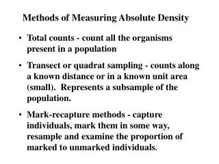
T. Kosztołowicz, Measuring subdiffusion parameters • Introduction. • Measuring subdiffusion parameters: • a) In the system with pure subdiffusion: • Anomalous time evolution of near-membrane layers • b) In the subdiffusive system with chemical reactions: • Anomalous time evolution of reaction front • c) In electrochemical system: • Anomalous impedance • Biological application: • Transport of organic acids and salts in the tooth enamel • Final remarks
Subdiffusion - subdiffusion parameter - subdiffusion coefficient Subdiffusion equation
glass cuvette aqueous solution of agarose 130 mm membrane laser beam aqueous solution of agarose and glucose Measuring subdiffusion parameters T. Kosztołowicz, K. Dworecki, S. Mrówczyński, PRL 94, 170602 (2005) Schematic view of the membrane system
Near-membrane layer (0,) Initial condition
Boundary conditions at the thin membrane 1. 2. ? or ?
The experimentally measured thickness of near-membrane layer as a function of time t for glucose with =0.05 (), =0.08 (), and =0.12 () and for sucrose with =0.08 (). The solid lines represent the power function At0.45.
Transport of glucose and sucrose in agarose gel For glucose: A = 0.091 ± 0.004 for = 0.05, = 0.45 A = 0.081 ± 0.004 for = 0.08, = 0.45 A = 0.071 ± 0.004 for = 0.12, = 0.45 = 0.90, D0.90 = (9.8 ± 1.0) 10–4 mm2/s0.90 For sucrose: A = 0.064 ± 0.003 for = 0.08, = 0.45 = 0.90, D0.90 = (6.3 ± 0.9) 10–4 mm2/s0.90
MEASUREMENT IN NON-TRANSPARENT MEDIUM theory T. Kosztołowicz, AIP 800 (2005) experiment K. Dworecki, Physica A 359, 24 (2006) PEG2000 in polyprophylene membrane, 180A pore size, 9x10⁹ pores/cm2
Subdiffusion-reaction system CA(x,0) = C0AH(-x) CB(x,0) = C0BH(x)
Time evolution of reaction front in subdiffusive system 1. DA= DB S.B. Yuste, L. Acedo, K. Lindenberg, PRE 69, 036126 (2004) T. Kosztołowicz, K. Lewandowska cond-mat/0603139 (2006) Phys. Rev. E (submitted) 2. DA DB , DA, DB > 0 T. Kosztołowicz, K. Lewandowska Acta Phys. Pol. 37, 1571 (2006) 3. DA > DB = 0
The schematic view of the tooth enamel The dotted line represents the concentration of static hydroxyapatite Ca5(PO4)3, the dashed one – the concentration of organic acid HB.
Lesion depth versus time The squares represent experimental data (J. Featherstone et al., Arch. Oral Biol. 24, 101 (1979) ), solid line is the plot of the power function xf = 0.39 t 0.32 . Since xf = Df t /2 , we obtain = 0.64.
A. Compte, R. Metzler, J. Phys. A 30, 7277 (1997) generalized Cattaneo equation
THE EXPERIMENTAL SETUP Impedance is measured using Solartron Frequency Response Analyzer 1360 and Biological Interface Unit 1293 in the frequency range 0.1 Hz to 100 kHz. Amplitude of signal was selected for 1000 mV.
EXPERIMENTAL RESULT = 0.30 ± 0.06
Final remarks • We have developed a method to extract the subdiffusion parameters from experimental data. The method uses the membrane system, where the transported substance diffuses from one vessel to another, and it relies on a fully analytic solution of the fractional subdiffusion equation. We have applied the method to the experimental data on glucose and sucrose subdiffusion in a gel solvent. • We show that the reaction front evolves in time as xf~Dft /2 with 1. The relation can be used to identify the subdiffusion and to evaluate the subdiffusion parameter in a porous medium such as a tooth enamel.
Final remarks • Our first method to determine the subdiffusion parameters relies on the time evolution of near-membrane layer =At/2. Why the parameters are not extracted directly from concentration proflies? There are some reasons to choice the near-membrane layers: • The near-membrane layer is free of the dependence on the boundary condition at the membrane • When the concentration profile is fitted by a solution of subdiffusion equation, there are three free parameters. When the temporal evolution of is discussed, is controlled by time dependence of (t) while D is provided by the coefficient A.
Fractional derivative ................................................................
Fractional integral ................................................................
Fractional derivatives and integrals The Riemann-Liouville (RL) definition K.B. Oldham, J. Spanier, The fractional calculus, AP 1974
Properties of fractional derivatives Linearity Chain rule Leibniz’s formula
Quasistationary approximation (for normal diffusion-reaction system Z. Koza, Physica A 240, 622 (1997), J. Stat. Phys. 85, 179 (1996)) Inside the depletion zone: In the region where R(x,t) ≈ 0
Measuring subdiffusion parameters Short history • Observing single particle • Single particle tracking D.M. Martin et al. Biophys. J. 83, 2109 (2002), P.R. Smith et al., ibid. 76, 3331 (1999) • Fluorescence correlation spectroscopy P. Schwille et al., Cytometry 36, 176 (1999) • Magnetic tweezers F. Amblard et al., PRL 77, 4470 (1996) • Optical tweezers A. Caspi, PRE 66, 011916 (2002) • Observing concentration profiles • NMR microscopy A. Klemm et al., PRE 65, 021112 (2002) • Anomalous time evolution of near membrane layer T. Kosztołowicz, K. Dworecki, S. Mrówczyński, PRL 94, 170602 (2005) • Anomalous time evolution of reaction front S.B. Yuste, L. Acedo, K. Lindenberg, PRE 69, 036126 (2004),T. Kosztołowicz, K. Lewandowska (submitted)
Subdiffusion equation Attention! so is not equivalent to
The same experimental data as in previous fig. on log-log scale. The solid lines represent the power function At0.45, the dotted lines correspond to the function At0.50.