Download
1 / 19
190 likes | 270 Views
The Model Photosphere (Chapter 9). Basic Assumptions Hydrostatic Equilibrium Temperature Distributions Physical Conditions in Stars – the dependence of T( t ), P g ( t ), and P e ( t ) on effective temperature and luminosity. Basic Assumptions in Stellar Atmospheres.

E N D
The Model Photosphere (Chapter 9) • Basic Assumptions • Hydrostatic Equilibrium • Temperature Distributions • Physical Conditions in Stars – the dependence of T(t), Pg(t), and Pe(t) on effective temperature and luminosity
Basic Assumptions in Stellar Atmospheres • Local Thermodynamic Equilibrium • Ionization and excitation correctly described by the Saha and Boltzman equations, and photon distribution is black body • Hydrostatic Equilibrium • No dynamically significant mass loss • The photosphere is not undergoing large scale accelerations comparable to surface gravity • No pulsations or large scale flows • Plane Parallel Atmosphere • Only one spatial coordinate (depth) • Departure from plane parallel much larger than photon mean free path • Fine structure is negligible (but see the Sun!)
Hydrostatic Equilibrium • Consider an element of gas with mass dm, height dx and area dA • The upward and downward forces on the element must balance: PdA + gdm = (P+dP)dA • If r is the density at location x, then dm= r dx dA dP/dx = g r • Since g is (nearly) constant through the atmosphere, we set g = GM/R2 P x gdm x+dx P+dP dP/dx = gr
In Optical Depth dP/dtn = g/kn • Since dtn=kn rdx • and dP=g rdx CLASS PROBLEM: • Recall that for a gray atmosphere, For k=0.4, Teff=104, and g=2GMSun/RSun2, compute the pressure, density, and depth at t=0, ½, 2/3, 1, and 2. (The density r and pressure equal zero at t=0 and k =1.38 x 10⁻¹⁶ erg K-1)
In Integral Form - • The differential form: • x Pg½ (where k0 is kn at a reference wavelength, typically 5000A) • Then integrate:
Procedure • Guess at Pg(tn) • Guess at T(tn) • Do the integration, computing kn at each level from T and Pe • This gives a new Pg(tn) • Interate until the change in Pg(tn) is small
The T(t) Relation • In the Sun, we can use • Limb darkening or • The variation of In with wavelength • to get the T(t) relation • Limb darkening can be described from: • We have already considered limb darkening in the gray case, where
The Solar T(t) Relation • So one can measure In(0,q) and solve for Sn(tn) • Assuming LTE (and thus setting Sn(tn)=Bn(T)) gives us the T(t) relation • The profiles of strong lines also give information about T(t) – different parts of a line profile are formed at different depths.
The T(t) Relation in Other Stars • Use a gray atmosphere and the Eddington approximation • More commonly, use a scaled solar model: • Or scale from published grid models • Comparison to T(t) relations iterated through the equation of radiative equilibrium for flux constancy suggests scaled models are close
DON’T Scale Pg(t)! Models at 5000 K
Computing the Spectrum • Now can compute T, Pg, Pe, k at all t (Pe=NekT) • Does the model photosphere satisfy the energy criteria (radiative equilibrium)? • Compute the flux from • Express In in terms of the source function Sn, and adopt LTE (Sn =B(T))