Download

1 / 44
440 likes | 645 Views
Chapter 16 Game Theory and Oligopoly. Figure 16.1 The monopoly equilibrium. The monopoly equilibrium. This chapter uses the following linear market demand curve: p=100-y Assume that each firm in the industry has a marginal/average/unit cost of $40. MR= 100-2y

E N D
The monopoly equilibrium • This chapter uses the following linear market demand curve: p=100-y • Assume that each firm in the industry has a marginal/average/unit cost of $40. • MR= 100-2y • Profits are maximized by charging the price associated with the optimal level of output -the level of output where MR=MC. • Total profits (TP) = TR – TC.
Duopoly as a Prisoner’s Dilemma • A Duopoly is an oligopoly in which there are only two firms in the industry.
From Table 16.1 • L is the dominant strategy for both the First and the Second Firm • Thus, the Nash-equilibrium combination is (L, L) in which both firms produce 20 units and have a profit of $200. • Yet, if they could agree to restrict their individual outputs to 15 units a piece, each could earn $450.
The Oligopoly Problem • Oligopolists have a clear incentive to collude or cooperate. • Oligopolists have a clear incentive to cheat on any simple collusive or cooperative agreement. • If an agreement is not a Nash equilibrium, it is not self-enforcing.
The Cournot Duopoly Model • Central features of the Cournot Model: • Each firm chooses a quantity of output instead of a price. • In choosing an output, each firm takes its rival’s output as given.
From Figure 16.2 • The First firm’s best response function is: y1*=30 – y2/2 • The Second firm’s best response function is y2*=30 – y1/2 • Taken together, these two best response functions can be used to find the equilibrium strategy combination for Cournot’s model.
The Cournot Model: Key Assumptions • The profit of one firm decreases as the output of the other firm increases (other things being equal). • The Nash equilibrium output for each firm is positive.
Isoprofit Curves • All strategy combinations that give the first firm the chosen level of profits is known as an indifference curve or isoprofit curve. • Profits are constant along the isoprofit curve.
From Figure 16.4 • y1* maximizes profits for the first firm, given the second firm’s output of y2*. • Any strategy combinations below the isocost curve gives the first firm more profit than the Nash equilibrium. • The result above relates to the key assumption that the first firm’s profit increases as the second firm’s output decreases.
Cournot’s Model: Conclusions • In the Nash equilibrium of this general version of the Cournot model, firms fail to maximize their joint profit. • Relative to joint profit maximization, firms produce too much output in the Nash equilibrium.
The Cournot Model with Many Firms • With only one firm in the market, the Cournot-Nash equilibrium is the monopoly equilibrium. • As the number of firms increase, output increases. As a result, price and aggregate oligopoly profits decrease. • When there are infinitely many firms, the Cournot model is, in effect, the perfectly competitive model.
The Cournot Model with Compliments • The Cournot-Nash equilibrium in which firms produce the same good is not Pareto-optimal, as the firms produced too much. • The Cournot-Nash equilibrium in which firms produce complements is not Pareto-optimal, as the firms produced too little.
The Bertrand Model • The Bertrand model substitutes prices for quantities as the variables to be chosen. • The goal is to find the Nash (the Bertrand-Nash) equilibrium strategy combination when firms choose prices instead of quantities.
The Bertrand Model: Firm’s Best Response Function • Finding the best response function entails answering the question: Given p2, what value of p1 maximizes the first firm’s profit. • Four possibilities exist: 1. If its rival charges a price greater than the monopoly price (MP), the first firm’s best response is to charge a lower price (than MP) so it can capture the entire market.
The Bertrand Model: Firm’s Best Response Function 2.If its rival charges a price less than the per unit cost of production (p2), the first firm’s best response is to choose any price greater than this because firm one will attract no business and incur a zero profit. This outcome is superior to matching or undercutting p2, and posting losses.
The Bertrand Model: Firm’s Best Response Function 3. If the second firm’s price is greater than the per unit cost of production and less than the monopoly price. • If p1< p2,the first firm captures the entire market and its profits increase as its price increases. • When p1= p2, the two firms split the profit. • When p1> p2, the first firm’s profit is zero because it sells nothing when its price exceeds the second firm’s price. (see Figure 16.6).
The Bertrand Model: Firm’s Best Response Function 4. Suppose the second firm sets its price exactly equal to the per unit costs. • Then if the first firm sets a lower price it will incur a loss on every unit it sells and profits will be negative. If the first firm sets a price above the per unit, it will sell no units and profits are zero. If the first firm sets price equal to the per unit costs, it breaks even.
The Bertrand-Nash Equilibrium • The Bertrand-Nash equilibrium strategy combination has the second firm and the first firm charging a price equal to the per unit cost of production. • At this equilibrium, each firm’s profit is exactly zero.
The Collusive Model of Oligopoly • The collusive model of oligopoly is when oligopolists decide to collude on a joint strategy. • In the Cournot and Bertrand models, the equilibriums are individually rational but collectively irrational, as firms have a clear incentive to collude. • However, if firms do manage to form a collusive agreement, there is a clear private incentive for each party to cheat.
The Collusive Model of Oligopoly • In the Cournot model, the individual incentive to cheat on the collusive agreement increases as the number of parties to the agreement increases. • This means that the larger the number of firms in an industry, the less likely is a collusive equilibrium. • If the number of firms is large enough, some firm or firms will succumb to the temptation to cheat, thereby destroying the collusive agreement.
Experimental Evidence • Taken together, experiments suggest that no single model is applicable to all oligopoly situations. • Perhaps the most economists can hope for is a selection of oligopoly models, each applicable to a particular range of economic circumstances.
The Limited-Output Model • In the long run, the number of firms (market structure) is endogenous. • The number of firms in an industry is determined by economic considerations. • The key process in determining the long-run equilibrium is the possibility of entry.
The Limited Output Model • Limited output models or limited price models focus on the theory of the oligopoly in the long run, where the number of firms is determined endogenously and there is the possibility of entry.
Barriers to Entry • A natural barrier to entry is setup costs. • Assume all firms incur setup costs of $S • In any period, the rate of interest (i) determines the set up cost (K):K=iS • Adding fixed costs to variable costs (40y) gives total cost function: C(y)=K+40Y
Inducement to Entry • If the fixed costs (K) are a barrier to entry, what is an inducement to entry? • An inducement to entry is the excess of revenue over variable costs.
Inducement to Entry • The entrant’s best response function is: yE*=30-y/2 • The entrant’s residual demand function is: Pe=(100-y)-ye • The price that will prevail if the entrant produces ye* units is: Pe*=70-y/2 • Profit per unit is: Pe* - 40=30-y/2
Inducement to Entry • The inducement to entry, ye* times (pe*-40) is then (30-y/)2. • This expression gives the revenue over variable costs that the entrant would earn if established firms continued to produce y units after entry. • Entry will occur if inducement to enter exceeds K.
Inducement to Entry • Call the smallest value of y, such that no entry occurs, the limit output (yL). • (30-yL/2)2=K • Solving for YL: YL= 60-2K1/2 • If K=$100, YL=40 units, If K=$225, YL=30 units, etc. • (see Figure 16.8)
Inducement to Entry • The no entry condition says entry will not occur if the output of established firms is greater than or equal to the limit output (yL) • The limit price (pL) is the price associated with the limit output. • In this example: pL=100-yL or pL= 40+2K1/2
Figure 16.8 Identifying the limit price and the limit output
Strategic Choice of Industry Output • The existing level of industry output (y) and development costs (K) are barriers to entry. • If y is less than the limit output yL, the firm will enter the industry. • If y is equal to or more than the limit output yL, the firm will not enter the industry.
Strategic Choice of Industry Output • We have calculated that if K=$225, then yL=30 (the monopoly output). • Thus, if setup costs are $225 or higher, the monopoly output of 30 will successfully deter entry – a natural monopoly scenario.
Strategic Choice of Industry Output • If K< $225, the ordinary monopolist output will not deter entry (yL>30). • In this case the monopolist will produce exactly yL units of output. • Since it has already incurred the setup cost, its objective is to maximize revenues over variable costs (gross profits).
Critique of the Model • The postulate that entrants take the current industry output as a given is the major weakness of the limited-output model. • A potential entrant’s concern is not with present but the future output of the sitting (currently in the industry) monopolist.
Critique of the Model • When a sitting monopolist produces the limit output, its decision is intended as a credible warning to potential entrants that it will continue to produce the limit output in the future. • If entrants take this warning seriously, they will stay out of the market.