Finite Element Method

1. Finite Element Method

2. FEM Approaches There are two main methods that are applied to solving problems using the FEM method. Variational methods that use the classical Rayleigh-Ritz technique Galerkin’s methods which is one technique in a family of methods referred to as method of weighted residuals.

3. Variational Approach In solving problems arising in physics and engineering it is often possible to replace the problem of integrating a differential equation by the equivalent problem of seeking a function that gives a minimum value of some integral. Problems of this type are called variational problems. The methods that allow us to reduce the problem of integrating a differential equation to the equivalent variational problem are usually called variational methods.

4. Variational Approach What is a functional? functional subjected to the boundary conditions • Goal: Find a function F(x,y,y’) for which the functional I(y) has an extremum (usually a minimum)

5. Variational Approach Some problems: NOT: • Question: Are there situations in which the function F(x,y,y’) for which the functional I(y) in minimized is ALSO a solution to the PDE and BCs??

6. Variational Approach • Question: Are there situations in which the function F(x,y,y’) for which the functional I(y) in minimized is ALSO a solution to the PDE and BCs?? • Answer: Yes, all PDEs typically found in physics and engineering have functionals or variational equations whose solution is equivalent to solving the PDE directly.

7. Variational Approach • Answer: Yes, all PDEs typically found in physics and engineering have functionals or variational equations whose solution is equivalent to solving the PDE directly. • Deriving those equations can be done using the calculus of variations (beyond the scope of this class).

8. Variational Approach

9. Finite Element Method The finite element method (FEM) has its origin in the field of structural analysis. However, since then the method has been employed in nearly all areas of computational physics and engineering. The FEM method, while more difficult to program than either the finite difference (FD) or method of moments (MOM), is a more powerful and versatile numerical technique for handling problems involving complex geometries and inhomogeneous media.

10. Basic concept Although the behaviour may be complex when viewed over a large region, a simple approximation may suffice over a small subregion. The region is divided up into finite elements. (usually, triangles or squares, but can be more complicated) Regardless of the shape the field is approximated by a different expression over each element, maintaining continuity at adjoining elements.

11. Solution Strategy: Variational Approach The equations to be solved are usually stated not in terms of field the variables but in terms of an integral-type functional such as energy. The functional is chosen such that the field solution makes the functional stationary The total functional is the sum of the integral over each element

12. Finite Element Method The finite element method (FEM) involves basically four steps: • Discretize the solution region into a finite number of subregions or elements • Derive the governing equations for each element based on either a variational approach or Galerkin’s method • Assemble all the elements together in the solution space. • Solve the resulting system of equations

13. Finite Element Method CREATING THE MESH • Discretize the solution region into a finite number of subregions or elements

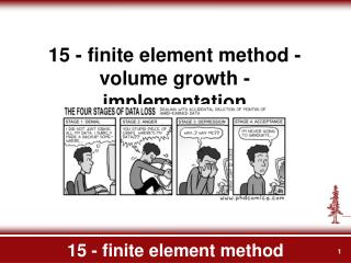
14. Finite Element Method in 2D CREATING THE MESH • Discretize the solution region into a finite number of subregions or elements • divide the geometry into elements • (in 2D triangular elements are common) • each element has a number of nodes • attached. • In this figure there are 8 elements (E1-E8) • and 9 nodes (N1-N9)

15. Finite Element Method The mesh is often described using two tables (element table and a node table) Element Table Element# Node1 Node2 Node3 1 4 7 8 2 4 8 5 3 8 9 5 ...... 8 2 6 3 Node Table Node# x y 1 0 1 2 0.5 1 3 1 1 ...... 9 1 0

16. y 2 x h 1 h 0 2D FEM: Right Triangular Single Element The simplest element is the right triangle (0,1,2) The potential can be calculated as a,b,c unknown ! Smart to specify the interpolation at the vertices! Then:

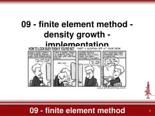
17. 6 7 3 0 2 1 4 5 8 Other elements Square element: consider as two triangles. This is ok, but does not lead to a smooth interpolation over the square. Better to use a higher order interpolation that uses four nodal values This scheme leads to:

18. Element expansion In general we wish to approximate the unknown function, (x,y), Inside an element by an interpolation of its values at the vertices. Number of vertices Provided the values at the vertices are known unknown anywhere within the element element shape functions or basis functions. In FEM these are usually interpolation functions

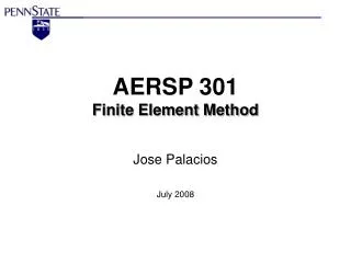
19. Generalized Triangular Develop the Governing Equations for a Single Element y Ve3 (x3, y3) Assume the unknown variable (V), in each element can be found as a linear interpolation of its value at the three nodes. FIND a, b and c 3 Ve2 (x2, y2) 2 Ve(x,y) 1 Ve1 (x1, y1) x

20. Finite Element Method Develop the Governing Equations for a Single Triangular Element y Ve3 (x3, y3) 3 Ve2 (x2, y2) 2 Ve(x,y) 1 Solve for the unknowns (a, b and c) and then substituting that result into Ve1 (x1, y1) x

21. Shape or basis functions (only function of geometry) Finite Element Method y Ve3 (x3, y3) 3 Ve2 (x2, y2) where 2 Ve(x,y) 1 Ve1 (x1, y1) x

22. Finite Element Method y Ve3 (x3, y3) 3 Ve2 (x2, y2) 2 Ve(x,y) 1 Ve1 (x1, y1) Properties of the shape functions x

23. 2D Example:Laplace’s Equation When the quantity being sought (here the electrostatic potential V) Recall: The true potential is known to minimize the electrostatic field energy.

24. 1 2 3 4 Create the Mesh Step #1: Discretize the surface/volume to be solved into small finite elements. Label each element and its associated nodes 1 2 3

25. 1 2 3 3 1 2 4 Basic concept: Review Step #2: Approximate the complex solution within the whole regionin terms of a sum of solutions found within each element

26. (x1,y1) (x3,y3) Element (x2,y2) FEM Laplace’s Equation Approximate the solution within each element in terms ofeach value at the corresponding nodes. (i.e. interpolation)

27. Finite Element Method To derive an equation for each element we plug in our linear approximation into an functional expression. y Ve3 (x3, y3) 3 Ve2 (x2, y2) 2 Ve(x,y) 1 Ve1 (x1, y1) x

28. Finite Element Method To derive an equation for each element we plug in our linear approximation into an functional expression. y Ve3 (x3, y3) 3 Ve2 (x2, y2) 2 Ve(x,y) 1 Ve1 (x1, y1) x

29. y Ve3 (x3, y3) 3 Ve2 (x2, y2) 2 Ve(x,y) 1 Ve1 (x1, y1) x Finite Element Method Example: Laplace’s Equation Let element coefficient matrix where and

30. y Ve3 (x3, y3) 3 Ve2 (x2, y2) 2 Ve(x,y) 1 Ve1 (x1, y1) x Finite Element Method Solution for triangular elements Example: Laplace’s Equation

31. y Ve3 (x3, y3) 3 Ve2 (x2, y2) 2 Ve(x,y) 1 Ve1 (x1, y1) x Finite Element Method Main property of the coefficient matrix:

32. Finite Element Method Assembling of All Elements Together Solve for the unknowns (a, b and c) and then substituting that result into where Global coefficient matrix and

33. Finite Element Method Assembling of All Elements Together 2 4 5 E1 1-4-2 (1-2-3) E3 3-5-4 (1-2-3) E2 1-3-4 (1-2-3) Coefficients are only non-zero for elements that touch each other 3 1

34. Finite Element Method Setting up and solving the resulting equations The solution for the node values is the ones that result in the functional obtaining its minimum value!

35. Finite Element Method Setting up and solving the resulting equations Example for five nodes:

36. Finite Element Method Setting up and solving the resulting equations Example for five nodes: In general:

37. Iterative solution method At node k in a mesh with n nodes, we have the solution e.g. see previous slide We note that Cki = 0 if node k is not directly connected to node i, only nodes that are directly connected to node k contribute to Vk. We apply this iteratively to all free nodes (not at fixed boundary value) where the potential is unknown. Initially we assign either 0, random or some average value to each free node and then iterate on the above equation until convergence is met.

38. Finite Element Method Example: Poisson’s Equation Equations for single element:

39. Finite Element Method Example: Poisson’s Equation Equations for single element: where and

40. Finite Element Method Example: Poisson’s Equation Equations for single element: Solution for triangular elements Solution for triangular elements

41. Finite Element Method Example: Poisson’s Equation Put all the elements together: Construct matrix and then solve:

42. Finite Element Method Example: Poisson’s Equation Example: Result in: In General:

43. Finite Element Method Example: Homogenous Wave Equation Equations for single element:

44. Finite Element Method Example: Wave Equation Equations for single element: where and

45. Finite Element Method Example: Wave Equation with no sources Equations for single element: where and

46. Finite Element Method Example: Wave Equation Put all the elements together:

47. Finite Element Method: Waveguide TM Modes TE Modes where y and x z

48. Finite Element Method: Waveguide TM Modes Put all the elements together: Band Matrix Solution: Break the matrices up into sub-matrices that distinguishes free-nodes from those that are known or prescribed nodes (i.e. boundary values):

49. Finite Element Method: Waveguide TM Modes Minimize the functional:

50. Finite Element Method: Waveguide TM Modes since tangential E field must vanish on PEC boundary For TM modes: