Dynamic regression with exponentially decreasing coefficients in the transfer function

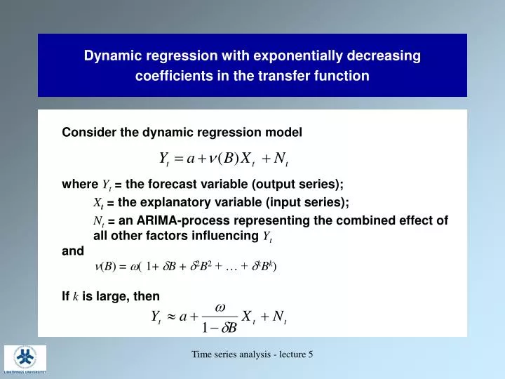
1. Dynamic regression with exponentially decreasingcoefficients in the transfer function Consider the dynamic regression model where Yt = the forecast variable (output series); Xt = the explanatory variable (input series); Nt = an ARIMA-process representing the combined effect of all other factors influencing Yt and (B) = ( 1+ B + 2B2 + … + kBk) If k is large, then Time series analysis - lecture 5

2. Parsimonious parameterization of dynamic regression models where Yt = the forecast variable (output series); Xt = the explanatory variable (input series); Nt = an ARIMA-process representing the combined effect of all other factors influencing Yt Important special cases: s = 0 and r = 0 Time series analysis - lecture 5

3. Selecting the order of a general dynamic regression model- values to be determined We need to determine: • the values of r, s, and b • the values of p, d, and q in the ARIMA(p, d, q) model of the noise Nt • the values of P, D, and Q of a seasonal ARIMA model, if such data are analysed Time series analysis - lecture 5

4. Selecting the order of a general dynamic regression model- LTF identification Step 1: Fit a multiple regression model with a low order AR model for the noise Step 2: If the errors from the regression appear to be non-stationary, then difference Y and X Step 3: Determine b, r, and s by inspecting the -weights in the regression Step 4: Compute the series of noise terms and fit an ARMA-model to these terms Step 5: Refit the entire model using the new ARMA model for the noise Time series analysis - lecture 5

5. Proc ARIMA in SAS –stationary inputs and outputs procarima data=timeseri.gasfurnace; identify var=CO2 crosscorr=gasrate; estimate p=1 input=(3$/(1)gasrate); run; Time series analysis - lecture 5

6. Proc ARIMA in SAS- nonstationary inputs and outputs procarima data=timeseri.gasfurnace; identify var=CO2 (1) crosscorr=gasrate(1); estimate p=1 input=(3$/(1)gasrate); run; Time series analysis - lecture 5

7. Intervention analysis where Yt = the forecast variable (output series); Xt = a step or pulse function; Nt = the combined effect of all other factors influencing Yt(the noise); (B) = (0 + 1B + 2B2 + … + kBk), wherekis the order of the transfer function Time series analysis - lecture 5

8. Intervention analysis- delayed or decayed response Delayed response: Xt is a step function Decayed response: Xt is a pulse function Time series analysis - lecture 5

9. Statistical methods for trend detection Concordant pair • Linear regression • Smoothing techniques • Non-parametric tests Discordant pair Concordant pair Time series analysis - lecture 5

10. The classical Mann-Kendall test for monotone trend in a single time series of data Test statistic: where Under H0, the test statistic T is approximately normal with mean zero and variance one Basic idea: Consider all pairs (Xi, Xj) of observations. Subtract the number of “discordant pairs” from the number of “concordant pairs” Time series analysis - lecture 5

11. Mann-Kendall tests for monotone trends in data collected over several seasonsCorrection for short-term serial dependence Hirsch&Slack (1984): Compute a Mann-Kendall statisticTjfor each seasonj=1,…,mand form T=T1+…+Tm Derive the variance ofTby using the Dietz-Killeen estimator of the covariance matrix of (T1,…,Tm) Time series analysis - lecture 5

12. Mann-Kendall tests for monotone trends in data collected at several sitesCorrection for dependence between sites Loftis et al. (1991): Compute a Mann-Kendall statisticTjfor each sitej=1,…,mand form T=T1+…+Tm Derive the variance ofTby using the Dietz-Killeen estimator of the covariance matrix of (T1,…,Tm) Time series analysis - lecture 5

13. From multiple time series of data to a smooth trend surface Time series analysis - lecture 5

14. A simple model for simultaneous smoothingand adjustment for a single covariate Let be the observed response for the jth coordinate the ith year, and let denote a contemporaneous value of a covariate. Assume that . Response Deterministic trend Impact of covariate Random error Time series analysis - lecture 5

15. A semiparametric model for simultaneous smoothingand adjustment for several covariates Let be the observed response for the jth class the ith year, and let denote contemporaneous values of covariates. Assume that . Random error Response Deterministic trend Impact of covariate Impact of covariate Time series analysis - lecture 5

16. Gradient smoothing . Penalty of irregular interannual variation Penalty of irregular variation along the gradient Time series analysis - lecture 5

17. Smoothing of the trend function in models of time series data representing several sites along a gradient Spatial smoothing along a gradient Temporal smoothing across years Time series analysis - lecture 5

18. Smoothing of the trend function in models of time series data representing several seasons Sequential smoothing across seasons Temporal smoothing across years Time series analysis - lecture 5

19. Smoothing of the trend function in models of time series data representing several sectors Circular smoothing across sectors Temporal smoothing across years Time series analysis - lecture 5

20. Total phosphorus concentrations atDagskärsgrund in Lake Vänern Time series analysis - lecture 5

21. Detection of an unknown level shift- the Standard Normal Homogeneity Test Let X1, …, Xn be a sequence of independent normal random variables with variance one H0: E(Xj) = 0 for 1  j  n H1: E(Xj) = 1 for j  m E(Xj) = 2 for j > m Test statistic where and are the average responses before and after the shift Time series analysis - lecture 5

22. Detection of a level shift and change-point detection Time series analysis - lecture 5

23. Total phosphorus concentrations atDagskärsgrund in Lake Vänern-simultaneous smoothing and change-point detection Time series analysis - lecture 5

24. Ratio between TOC (total organic carbon) and permanganate consumption in Swedish rivers Time series analysis - lecture 5

25. Ratio between TOC (total organic carbon) and permanganate consumption in Swedish rivers- simultaneous smoothing and change-point detection Time series analysis - lecture 5

26. Uncertainty assessment and hypothesis testing in joint models of smooth trends and change-points • Resampling techniques are needed • Standard resampling techniques must be modified to accommodate correlated residuals Time series analysis - lecture 5