Download
1 / 81
820 likes | 1.08k Views
Log-Linear Models in NLP. Noah A. Smith Department of Computer Science / Center for Language and Speech Processing Johns Hopkins University nasmith@cs.jhu.edu. Outline. Maximum Entropy principle Log-linear models Conditional modeling for classification Ratnaparkhi’s tagger

E N D
Log-Linear Models in NLP Noah A. Smith Department of Computer Science / Center for Language and Speech Processing Johns Hopkins University nasmith@cs.jhu.edu
Outline • Maximum Entropy principle • Log-linear models • Conditional modeling for classification • Ratnaparkhi’s tagger • Conditional random fields • Smoothing • Feature Selection
Data For now, we’re just talking about modeling data. No task. How to assign probability to each shape type?
Maximum Likelihood Fewer parameters? How to smooth? 11 degrees of freedom (12 – 1).
Size Shape Some other kinds of models 11 degrees of freedom (1 + 4 + 6). Color These two are the same! These two are the same! Pr(Color, Shape, Size) = Pr(Color) • Pr(Shape | Color) • Pr(Size | Color, Shape)
Size Shape Some other kinds of models 9 degrees of freedom (1 + 2 + 6). Color Pr(Color, Shape, Size) = Pr(Color) • Pr(Shape) • Pr(Size | Color, Shape)
Size Shape Some other kinds of models 7 degrees of freedom (1 + 2 + 4). Color No zeroes here ... Pr(Color, Shape, Size) = Pr(Size) • Pr(Shape | Size) • Pr(Color | Size)
Size Shape Some other kinds of models 4 degrees of freedom (1 + 2 + 1). Color Pr(Color, Shape, Size) = Pr(Size) • Pr(Shape) • Pr(Color)
This is difficult. Different factorizations affect: smoothing # parameters (model size) model complexity “interpretability” goodness of fit ... Usually, this isn’t done empirically, either!
Desiderata • You decide which features to use. • Some intuitive criterion tells you how to use them in the model. • Empirical.
Maximum Entropy “Make the model as uniform as possible ... but I noticed a few things that I want to model ... so pick a model that fits the data on those things.”
Occam’s Razor One should not increase, beyond what is necessary, the number of entities required to explain anything.
Pr( , small) = 0.048 0.048 0.625
Pr(large, ) = 0.125 0.048 ? 0.625
Questions Is there an efficient way to solve this problem? Does a solution always exist? Is there a way to express the model succinctly? What to do if it doesn’t?
Entropy • A statistical measurement on a distribution. • Measured in bits. • [0, log2|X|] • High entropy: close to uniform • Low entropy: close to deterministic • Concave in p.
Max The Max Ent Problem H p2 p1
The Max Ent Problem objective function is H probabilities sum to 1 ... picking a distribution ... and are nonnegative expected feature value under the model n constraints expected feature value from the data
The Max Ent Problem H p2 p1
1 if x is a small , 0 otherwise About feature constraints 1 if x is large and light, 0 otherwise 1 if x is small, 0 otherwise
Max Mathematical Magic constrained |X| variables (p) concave in p unconstrained N variables (θ) concave in θ
What’s the catch? The model takes on a specific, parameterized form. It can be shown that any max-ent model must take this form.
Outline • Maximum Entropy principle • Log-linear models • Conditional modeling for classification • Ratnaparkhi’s tagger • Conditional random fields • Smoothing • Feature Selection
Log-linear models Log linear
Log-linear models One parameter (θi) for each feature. Unnormalized probability, or weight Partition function
Max Mathematical Magic Max ent problem constrained |X| variables (p) concave in p unconstrained N variables (θ) concave in θ Log-linear ML problem
What does MLE mean? Independence among examples Arg max is the same in the log domain
Iterative Methods All of these methods are correct and will converge to the right answer; it’s just a matter of how fast. • Generalized Iterative Scaling • Improved Iterative Scaling • Gradient Ascent • Newton/Quasi-Newton Methods • Conjugate Gradient • Limited-Memory Variable Metric • ...
Questions Is there an efficient way to solve this problem? Yes, many iterative methods. Does a solution always exist? Is there a way to express the model succinctly? Yes, if the constraints come from the data. Yes, a log-linear model.
Outline • Maximum Entropy principle • Log-linear models • Conditional modeling for classification • Ratnaparkhi’s tagger • Conditional random fields • Smoothing • Feature Selection
Conditional Estimation labels examples Training Objective: Classification Rule:
Maximum Likelihood label object
Maximum Likelihood label object
Maximum Likelihood label object
Maximum Likelihood label object
Conditional Likelihood label object
Remember: log-linear models conditional estimation
Log-linear models: MLE vs. CLE Sum over all example types all labels. Sum over all labels.
Classification Rule Pick the most probable label y: We don’t need to compute the partition function at test time! But it does need to be computed during training.
Outline • Maximum Entropy principle • Log-linear models • Conditional modeling for classification • Ratnaparkhi’s tagger • Conditional random fields • Smoothing • Feature Selection
Ratnaparkhi’s POS Tagger (1996) • Probability model: • Assume unseen words behave like rare words. • Rare words ≡ count < 5 • Training: GIS • Testing/Decoding: beam search
The “Label Bias” Problem (4) (6)
The “Label Bias” Problem Pr(VBN | born) Pr(IN | VBN, to) Pr(NN | VBN, IN, wealth) = 1 * .4 * 1 born to VBN, IN wealth VBN ■ IN, NN to run VBN, TO TO, VB Pr(VBN | born) Pr(TO | VBN, to) Pr(VB | VBN, TO, wealth) = 1 * .6 * 1 born to wealth