Download
1 / 73
730 likes | 868 Views
Genome Browsers for power users. The ENCODE project Up- and downloading data from the browser Analyzing genomic data in R (depending on time) Galaxy – a power user tool to interact with the browser. Some (almost) cutting edge science: The ENCODE project. Enc yclopedia O f D NA E lements

E N D
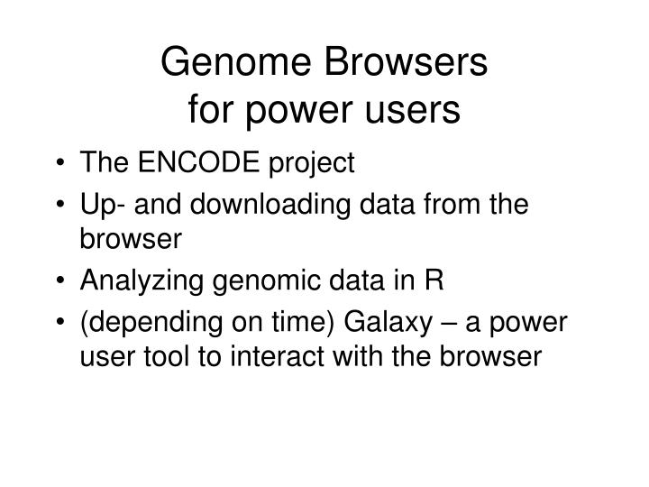
Genome Browsers for power users • The ENCODE project • Up- and downloading data from the browser • Analyzing genomic data in R • (depending on time) Galaxy – a power user tool to interact with the browser
Some (almost) cutting edge science:The ENCODE project • Encyclopedia Of DNA Elements • Aims for a targeted and coordinated elucidation of the (whole) human genome, using multiple systems • Currently ended the pilot phase: analyze 1% (30 Mbp)of the genome deeply • 44 regions • 14 regions chosen by function: for instance the HOXD gene cluster – 0.5 to 2 Mbp • 30 regions chosen “randomly” - 500 kb • Should be viewed as a pilot project for the rest of the genome – so both technology and biology is driving • A large number of labs involved in both data production and analysis
Some impressive numbers • 400 million data points, excluding sequencing of other genomes (adds another 250 million)! • Tiling arrays from 11 different cell sources • 96 ChIP-chip experiments • Tag sequencing data to identify promoters (covered later in the course) • In-depth cDNA annotation (GENCODE) • Sequencing of orthologous regions in a wide array of species • …and a lot more
Why introduce these things now in the course? • Get you used to look at tons of data at once • This is a fantastic data resource, which is under-used • make you realize that to analyze such data, you will have to understand the underlying method/biology • It will be 100* bigger in a year…
In this course 1: How to use the web interface; understanding the data types 2: How to download and upload data to the browser; interaction with R 3: How to make complex analyses between data types; Galaxy and R
Power users • As power users, we want to • Compare our OWN data with the annotations graphically • Download data and test hypothesis: the web browser is for casual viewing and dreaming up hypotheses! • Overlap different data types
For instance… • What genes are close to my new chip-data sites? • What is the conservation of these sites? • Do they overlap with other chip sites • Etc, etc • We will learn to do all this this week!
Uploading data • We can upload custom tracks in the browser - for instance, results of new experiments • To do this, we need to know what formats that the browser likes
BED • Block annotation - something starts and ends at certain positions (method of choice - more in next slide) • GFF • A standard annotation format in bioinformatics. Very similar to BED • GTF • Variant of GFF (I have never used this) • WIG • Format for continuous data - one “score” per nucleotide, or similar. Method of choice when BED is not a good option. Will touch on this. • PSL • An alignment format - the output of the BLAT program. Will not use this in the course.
BED A text file that in each line shows one “entity” that is mapped to the genome - a gene, a site for a factor, etc Can have up to 12 tab-separated columns, but only three are required: 1. chrom - The name of the chromosome (e.g. chr3, chrY). 2. chromStart - The starting position of the feature in the chromosome or scaffold. The first base in a chromosome is numbered 0. 3. chromEnd - The ending position of the feature in the chromosome or scaffold. The chromEnd base is not included in the display of the feature. For example, the first 100 bases of a chromosome are defined as chromStart=0, chromEnd=100, and span the bases numbered 0-99. Example: chr7 127471196 127472363 chr22 20100011 20100200
The name of the track • If we have many tracks, it really helps to have a name of each new track • We can start a bed file by a “track line” which gives name, description, plus some nice options (more later) • Can look like this track name=”Dataset 1" description=”Cell line X treatment” chr7 127471196 127472363 chr22 20100011 20100200
…so a small bed file could look like this track name=clones description=”There are many of me and we have a plan" chr22 10000000 10004000 chr22 10002000 10006000 chr22 10005000 10009000 chr22 10006000 10010000 chr22 10011000 10015000 chr22 10012000 10017000 Live Demo:I will just paste this into the browser “custom track” page
Reverse engineering challenge Example again: track name=clones description=”my Clones" chr22 10000000 10004000 chr22 10002000 10006000 chr22 10005000 10009000 chr22 10006000 10010000 Locate the RGS9 gene in the browser, assembly hg18 Can you make a bed file which exactly replicates the first exon (see example in next slide)? You have to find what the coordinates should be by zooming It should have the track name “my_refseq” (5 minutes)
track name=“my_refseq” description=”my_refseq" chr17 60564010 60564177 These coordinate are only meaningful with the May 2005 assembly
Challenge 2: real data At the web page, on today’s date, there is a link to a directory containing a bed file of chip-chip data of estrogen receptor alpha sites: ERA_mm8.bed (this is a text file!) These are from the mm8 assembly • Upload these to the browser with the correct assembly • Look at the following genes to see if they have one or more sites inside them or further upstream • Nrip1 • Esr1 (what is this gene?) • Hoxa1
track name="ERA" description="Estrogen receptor alpha" color=255,0,0 visibility=0 browser position chr6:28,912,411-28,925,620
The 9 additional optional BED fields are: 4. name - Defines the name of the BED line. 5. score - A score between 0 and 1000. If the track line useScore attribute is set to 1 for this annotation data set, the score value will determine the level of gray in which this feature is displayed (higher numbers = darker gray). 6. strand - Defines the strand - either '+' or '-'. 7. thickStart - The starting position at which the feature is drawn thickly (for example, the start codon in gene displays). 8. thickEnd - The ending position at which the feature is drawn thickly (for example, the stop codon in gene displays). 9. itemRgb - An RGB value of the form R,G,B (e.g. 255,0,0). If the track line itemRgb attribute is set to "On", this RBG value will determine the display color of the data contained in this BED line. NOTE: It is recommended that a simple color scheme (eight colors or less) be used with this attribute to avoid overwhelming the color resources of the Genome Browser and your Internet browser. 10. blockCount - The number of blocks (exons) in the BED line. 11. blockSizes - A comma-separated list of the block sizes. The number of items in this list should correspond to blockCount. 12. blockStarts - A comma-separated list of block starts. All of the blockStart positions should be calculated relative to chromStart. The number of items in this list should correspond to blockCount.
Genome graphs Gene density in the human genome - took < 2 minutes to do
Live demo: • Where are the ENCODE regions on the genome? • As you remember, the ENCODE regions are 1% of the genome – but what 1%?
Challenge • In the data directory, there is a set of estrogen alpha chip sites at the mm8 assembly (we used it some slides back). • Upload this to the mm8 browser (unless you already have) just as before (NOT via genome graph) • Then, import this set into the genome graph tool (under custom tracks) • What is your impressions? Where are they?
Downloading data • We often want to download whole data tracks to do analysis on them, in R • The table browser is a great tool to do this with • It allows for selecting tracks, or part of tracks, and also see the underlying data structure • Accessed by clicking on “Tables” on top of the browser
(with live demo: get all RefSeq genes from chromosome 1) Step 1. Pick a genome assembly (and species) Step 2. Pick an annotation track The group list shows all the annotation track groups available in the selected genome assembly. The names correspond to the groupings displayed at the bottom of the Genome Browser annotation tracks page. When a group is selected from the list, the track list automatically updates to show all the annotation tracks available within that group. * To examine all the tracks available within a certain group (e.g. all gene prediction tracks), select the group name from the group list, then browse the entries in the track list.
Step 3. Pick a table The table list shows all tables (both positional and non-positional) associated with the currently-selected track. By default, it displays the primary table for the track, i.e. the table containing the data shown in the Genome Browser annotation track. Other tables in the list are linked to the primary table by a common field and may provide supporting data used in constructing the annotation. Step 4. Pick a genomic region (positional tables only) By default, the Table Browser region is set to genome, which will display all the data records in the selected table.
What are we actually getting back? #bin name chrom strand txStart txEnd cdsStart cdsEnd exonCount exonStarts exonEnds id name2 cdsStartStat cdsEndStat exonFrames 585 NM_001005484 chr1 + 58953 59871 58953 59871 1 58953, 59871, 0 OR4F5 cmpl cmpl 0, 587 NM_001005224 chr1 + 357521 358458 357521 358458 1 357521, 358458, 0 OR4F3 cmpl incmpl 0, 587 NM_001005277 chr1 + 357521 358458 357521 358458 1 357521, 358458, 0 OR4F16 cmpl incmpl 0, 587 NM_001005221 chr1 + 357521 358460 357521 358460 1 357521, 358460, 0 OR4F29 cmpl cmpl 0, 589 NM_001005221 chr1 - 610958 611897 610958 611897 1 610958, 611897, 0 OR4F29 cmpl cmpl 0, 589 NM_001005224 chr1 - 610960 611897 610960 611897 1 610960, 611897, 0 OR4F3 incmpl cmpl 0, 589 NM_001005277 chr1 - 610960 611897 610960 611897 1 610960, 611897, 0 OR4F16 incmpl cmpl 0, 591 NM_152486 chr1 + 850983 869825 851184 869396 14 850983,851164,855397,856281,861014,864282,8 Slightly confusing! Lets go back to the table browser to get explanations
#bin name chrom strand txStart txEnd cdsStart cdsEnd exonCount exonStarts exonEnds id name2 cdsStartStat cdsEndStat exonFrames#bin name chrom strand txStart txEnd cdsStart cdsEnd exonCount exonStarts exonEnds id name2 cdsStartStat cdsEndStat exonFrames 585 NM_001005484 chr1 + 58953 59871 58953 59871 1 58953, 59871, 0 OR4F5 cmpl cmpl 0, 587 NM_001005224 chr1 + 357521 358458 357521 358458 1 357521, 358458, 0 OR4F3 cmpl incmpl 0, 587 NM_001005277 chr1 + 357521 358458 357521 358458 1 357521, 358458, 0 OR4F16 cmpl incmpl 0, 587 NM_001005221 chr1 + 357521 358460 357521 358460 1 357521, 358460, 0 OR4F29 cmpl cmpl 0, 589 NM_001005221 chr1 - 610958 611897 610958 611897 1 610958, 611897, 0 OR4F29 cmpl cmpl 0, 589 NM_001005224 chr1 - 610960 611897 610960 611897 1 610960, 611897, 0 OR4F3 incmpl cmpl 0, 589 NM_001005277 chr1 - 610960 611897 610960 611897 1 610960, 611897, 0 OR4F16 incmpl cmpl 0, 591 NM_152486 chr1 + 850983 869825 851184 869396 14 850983,851164,855397,856281,861014,864282,8
Analyzing downloaded data These are normal text files and can be read by R! Two handy tricks: • Give an output file names directly in the web form - some browsers try to save the html page otherwise (HTML has a lot of junk ><> signs) • After you have the file, remove the # in the first line, and you will get nice column names for the data, otherwise, this row will be ignored
Larger Challenge • Download all refseq genes from chr1, and chr2, from the mm8 assembly, to two different files. • Using R: • Make two vectors describing gene lengths from the different chromosomes • Hint: use end and start… • Are these significantly different in means/medians? Which chromosome has the longest genes?
c1<-read.table("refseq_mm8_chr1.txt", h=T) chr1_dist<-c1$txEnd-c1$txStart chr2_dist<-c2$txEnd-c2$txStart boxplot (chr1_dist, chr2_dist) boxplot (chr1_dist, chr2_dist, log=“y”) wilcox.test(chr1_dist, chr2_dist)
In this course 1: How to use the web interface; understanding the data types 2: How to download and upload data to the browser; interaction with R 3: How to make complex analyses between data types; Galaxy and R
The Galaxy tool • Galaxy is a user-friendly interface to power-user analysis of UCSC data • The main strength is that we can overlap tracks, make sub-tracks, and do some statistics WITHIN the browser • We can use this together with R for even more complex stuff
A different assignment setup… • The Galaxy people has made several very informative screencasts, which we will shamelessly steal • The general format is that we will watch a short video lecture showing a concept or technique. • You will then try to repeat the analysis - the video lecture you can play yourself if you need a recap: great way to prepare before home works • Later on, we will combine different things from different screencasts, and also explore things not covered in the casts
Where is galaxy? • See link on homepage, or • http://main.g2.bx.psu.edu/ • Please work in groups of 3 persons per computer (and connection) to not overload their server – we got thrown out last year
General intro to getting data to and from Galaxy and UCSC • UCSC2galaxy.mov • Objective: • 1) find all protein-coding exons and overlap them with all SNP data • 2) make these overlaps into a genome browser track
Try it out! • Objective: • (on chr22) • 1) find all protein-coding exons and overlap them with all SNP data • 2) make these overlaps into a genome browser track • Try to repeat this WITHOUT the screen cast and see how well you can manage • Use the screen cast if you get stuck
Manipulating data • text_manipulation.mov • We learn how to add columns and compute something on each entry
Try it out • Again, try it with the help of the screen cast to make an output file based on the coding exon table you imported that looks like this: • Chr Start End Your_Own _ID exon_length • Additional challenge (not covered by screen cast): • Using the Statistics option in the Toolbox, what is the mean exon length?
Intervals A set of screen casts showing things we can do with “intervals” • Getting the data • Genome coverage of a set • Coverage of one set to another • Intersects (recap), and subtractions betweens sets • Cluster the parts of a set
We will look at these casts in order, one by one, (all are in the sub-directory intervals): • data_prep.mov • base_cov_and_complement.mov • coverage.mov • intersect_and_subtract.mov • cluster.mov
Do it! • This is just to get the data to play with - should go fast! • Additional challenge: Upload the CpG islands track for later use • At the next cast, we will see how much of the genome that the different tracks cover