Download
1 / 61
610 likes | 771 Views
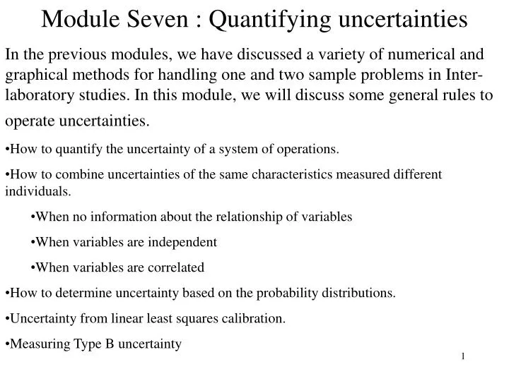
Module Seven : Quantifying uncertainties In the previous modules, we have discussed a variety of numerical and graphical methods for handling one and two sample problems in Inter-laboratory studies. In this module, we will discuss some general rules to operate uncertainties.

E N D
Module Seven : Quantifying uncertainties • In the previous modules, we have discussed a variety of numerical and graphical methods for handling one and two sample problems in Inter-laboratory studies. In this module, we will discuss some general rules to operate uncertainties. • How to quantify the uncertainty of a system of operations. • How to combine uncertainties of the same characteristics measured different individuals. • When no information about the relationship of variables • When variables are independent • When variables are correlated • How to determine uncertainty based on the probability distributions. • Uncertainty from linear least squares calibration. • Measuring Type B uncertainty
A system of components involving the measurement of uncertainty In many practical cases, we are interested in measuring the combined uncertainty of the entire system which consists of several uncertainty measurements. X1 X2 Xk Output Input The system consists of k components. Each component, we measure its uncertainty: Where is the best estimate for the component i. is the measurement uncertainty. The system is a function of ,denoted by
Four Questions involving quantifying the uncertainty of the system Q3: If there are n individuals measure the same component. Each obtains a measurement How do we combine these measurements and uncertainties ? Q1: When measuring the uncertainty of one variable, x. It is often that f(x) is the interest of measurement. How do we extend the measurement uncertainty to f(x), if the measurement of x with uncertainty is ? Q2: How to quantify the uncertainty of Our goal is to quantify in terms of
For each measurand, the measurement of the measured property usually obeys certain probability distribution. For example, a normal curve has been used for a variety of continuous variables. These distributional characteristics allow us to make a confidence interval estimate of the measurement with an intended level of confidence. Q4: When the distribution characteristic is applied to measuring the uncertainty, how to quantify the uncertainty based on the distribution characteristic of the measured property?
Q1: When measuring the uncertainty of one variable, x. It is often that f(x) is the interest of measurement. How do we extend the measurement uncertainty to f(x), if the measurement of x with uncertainty is ? f(x+Ux) f(x) f(x-Ux) f(x) f(x) Uf Uf f(x+Ux) f(x-Ux) x-Ux x x+Ux x-Ux x x+Ux Some common functions of x variable are Case 1: f(x) = axn Case 2: exp(x) We consider the general form of f(x) and apply to these special cases.
A fundamental calculus approximation asserts the following fact , given f(x) is monotone increasing, for Ux sufficiently small: This gives the uncertainty of f(x): , when f(x) is an increasing function of x. Similarly, when f(x) is decreasing, the uncertainty of f(x) is Combining these two situations, the measurement of f(x) with uncertainty is given by: Case 1: f(x) = xa : f(x) with uncertainty is Case 2: f(x) = exp(x): f(x) with uncertainty is Case 3: f(x) = ln(x): f(x) with uncertainty is Case 4: f(x) = cos(x): f(x) with uncertainty is Case 5: f(x) = ax: f(x) with uncertainty is
Examples: • One measured the thickness of 100 sheets of papers many times and obtain the thickness: • What is the thick ness of one sheet of paper? • Ans: f(x) =x/100. The thickness of one sheet is • One measured the radius of a circle and obtain the measurement: • What is the measurement of the area of the circle? • Ans: f(x) = pr2. The area is • Class Hands-on activity • Using the hands-on activity of ‘drawing 2 cm of line segment’ data to compute the uncertainty of your draws using the 10 data points, that is compute the sample s.d. Then, estimate the uncertainty for drawing one cm line segment.
Q2: How to quantify the uncertainty of Our goal is to quantify in terms of We begin with a simple system of two components, x and y The measurements and uncertainties are The basic function of f(x,y) for describing the system are Case 1: x + y Case 2: x-y Case 3: xy Case 4: x/y Any function that is a combination of these operations can be propagated.
Conditions of measuring uncertainty when combining variables: • No prior information about the components themselves or their relationship: For this situation, the maximum combined uncertainty may be more appropriate. • When variables are independent, that is the process of measuring one component is not related to the process of measuring other processes: For this situation, the independence property can be applied to reduce the combined uncertainty. • When distribution of the variables are known or can be approximated reasonably by some probability distributions, the measurement uncertainty of the component is estimated by standard error of the best estimate, and a probability of confidence can be obtained to describe the measurement uncertainty. Type A and Type B uncertainty are defined accordingly. • It often happens in a practical situation, uncertainty occurs not only randomly, but also systematically. One needs to be careful about the existence of systematic error, and make an effort to estimate this component of error, when ever possible. When reporting uncertainty involving both random error and systematic error, it is a good practice to provide separate presentation as well as combined uncertainty.
We have introduced Youden Plots and some numerical measures for measuring systematic and random errors. The estimation of systematic error requires some additional effort by conducting appropriate experiments that are specifically designed for estimating a suspected systematic error component. The analysis often depends on the design of the experiment. Some commonly used designs and their analysis will be discussed later. In this following we will focus on measuring measurement uncertainty for condition (1) and (2). Case 1: f(x,y) = x+y Given the uncertainty for each variable: We are looking for Under Condition 1: Maximum possible measurement for (x+y) is x+Ux + (y+Uy) = (x+y) +(Ux+Uy) The minimum possible measurement is (x+y) –(Ux+Uy) Therefore, the uncertainty for the sum is :
Case 1: Under Condition 2 : x and y are independent Independence of x and y has the following geometric property for the uncertainty: Uy Ux The uncertainty of x+y, due to independence, is given by U(x+y) = Case 1: Condition 3: x and y follow a certain probability distribution. The measurement of property x is the best estimate from the sample information (Type A) or from the physical property or prior knowledge (Type B). At first, step, we determine the best estimate for the characteristic by observing n measurements. The uncertainty of the variable x is estimated by sample standard deviation. In many cases, we are interested in estimating the unknown average of the characteristic. The best estimate is the sample mean, The uncertainty of is the Standard Error of , which is And is estimated by the sample standard deviation, sx.
The estimate of the average characteristic for variable x and its uncertainty is Similarly, the best estimate of the average for variable y and its uncertainty is Assuming that the two samples are chosen at random , and x and y are independent. Therefore, the uncertainty of the average of (x+y) is
Under Condition3: the best estimate and the uncertainty is: Case 2: f(x,y) = x-y: Under Condition 1: the uncertainty is Under Condition 2: the uncertainty is
Case 3: f(x,y) =xy Under Condition 1: x is measured by = x(1+ ) Therefore, the measurement of f(x,y) = xy is x * y = xy = xy(1+ + + ) (xy)(1+ + ) = xy (1+ ) Therefore, Case 3, Under Condition 2: X and Y are independent: The fractional uncertainty of f(x,y) = xy is given by
Case 4: f(x,y) = x/y: Under Condition 1: The largest measurement of f(x,y)= x/y = The smallest measurement of f(x,y)= x/y = Using the Binomial Expression: 1/(1-a) = 1+a+a2+a3+ …. When a is small, we can approximate 1/(1-a) = 1+a. The largest measurement of x/y has the form of (1+b)/(1-a) (1+b)(1+a) = 1+b+a+ab 1+a+b (since ab is very small). The largest measurement of x/y = Similarly, smallest measurement is Therefore, the measurement of x/y with uncertainty is Case 4: f(x,y)=x/y: Under Condition 2: The measurement of x/y with uncertainty is
Under Condition1: the measurement of f(x1,x2, …, xk) with uncertainty is given by: Under Condition 2: xi’s are independent. The measurement of f(x1,x2, …, xk) with uncertainty is given by: A General form of combining k variables, x1,x2, … xk. Case 1 to 4 are cases of combining two variables of x and y. Their measurement uncertainties are investigated under three different conditions for case 1 and 2,and under two conditions for case 3 and 4. In this section, we will consider a general function, f(x1,x2, …,xk)
Examples: • To find the area of a triangle, the base is measured to be • The height is measured to be • What is the measurement of the area? • Ans: f(b,h) = bh/2. Under condition 1: the fractional uncertainty of f(x) = • Hence, the area is • Under Condition 2: The measuring process of base and height are independent. • The fractional uncertainty of f(b.h) = • Hence, the area is
Hands-on Activity • Consider a system consists of four components: x,y,z,w. The measurements are • Suppose the system is • Find the measurement of f under condition 1 and 2. • (b) Suppose the system is • Find the measurement of f under condition 1 and 2. • ( c) Suppose the system is • Find the measurement of f under condition 1 and 2. • (d) Suppose the system is • Find the measurement of f under condition 1 and 2. • (e) Suppose the system is • Find the measurement of f under condition 1 and 2.
Under Condition1: the measurement of f(x1,x2, …, xk) with uncertainty is given by: Under Condition 2: xi’s are independent. The measurement of f(x1,x2, …, xk) with uncertainty is given by: A General form of combining k variables, x1,x2, … xk- Continued We discuss how to determine the uncertainty of a general function, f(x1,x2, …,xk) under Condition 1: no information is known, and (2) Variables are independent. There are situations where some variables may not be independent. For example, when measuring the water pressure of water in a container, it clearly related to the volume of the container. In some cases, the physical or chemical properties give us functional relations between variables, and we can take the advantages of the function relationship. In many, we do not have the functional relation. However, we can use data to estimate their relation and take into account the relation into the computation of combined uncertainty. Recall the results under conditions (1) and (2). When Xi’s are correlated, we need to estimate the correlation structure and take it into the computation of the uncertainty.
We shall consider several simple cases before discussing the general form for cases when variables are correlated. Case 1: f(x,y) = x +y. X and y are random variables follows a certain probability distribution. Then a typical measure of uncertainty is the variance. Result 1: V(x+y) = v(x) +v(y) + cov(x,y), where cov(x,y) is called the covariance of x and y. When samples are uses to estimate these components, v(x) is estimated by V(y) is estimated by And cov(x,y) is estimated by The standardize form of cov(x,y) gives the correlation coefficient, is estimated by the Pearson’s correlation:
For computational simplicity, we usually compute Sum of Squares and apply them to compute variances , covariance and correlation coefficient. From the correlation, the estimated covariance can be computed from correlation and sample variances: These formulae look pretty complicated. However, they all come from three values: SSx , SSy, and SSxy. The following figures demonstrate some cases of correlation.
Result 2: with xi’s being random variables The uncertainty is just the sample standard deviation of the corresponding estimate of the function when using sample information. Therefore, in terms of the uncertainty notation, result 2 becomes to: Result 3:
Measurement Uncertainty of a general function f(x1,x2, …,xk) with the xi’s being correlated. NOTE: When sample information is used to estimate the uncertainty, U(x) = sx , and U(x,y) = cov(x,y) = rxyU(x)U(y) = rxy(sx)(sy)
Hands-on activity A system consists of three components, x,y,z. These components are correlated. Based on the sample information, the sample variance-covariance matrix is The measurement for each component is: • Suppose the system is f(x,y,z) = 2x-y/z. • Determine the uncertainty for the system. • (b) Suppose the system is f(x,y,z) =(x/2 – y2)z • Determine the uncertainty for the system.
Consider the situation: Three standardized labs tested the same material using the same procedure and assume the environmental conditions are uniform. The tested results from the three labs are: The intend is to combine the testing results as the reference for other labs. This type of problem is different from what we discussed before. In this case, we measured one variables by three participants, and obtain different uncertainties. It is most likely that each result is from a repetitions of several tests. In this case, xj is the sample mean, and Uj is the standard deviation of mean, . Q3: If there are n individuals measure the same component. Each obtains a measurement How do we combine these measurements and uncertainties ?
In combining these results to obtain the best estimate, we should make sure that the lab testing results are consistent, and the lab systematic error is negligible. That is the uncertainty is from the random error only. Therefore, before combining the test results, we should make a quick check : • If there are any unusually large discrepancy |xi – xj| between each lab.If this discrepancy is much larger than Ui and Uj, we should suspect that at least one measurement has gone wrong, and a close examination of the process of testing is needed. • If there is any unusually large uncertainty from a lab. If Ui/Uj is over three, we should suspect some systematic errors exist, and a close examine of the process of testing is needed. One way to combine the testing results is by an average: f(x1,x2,x3) = (x1+x2+x3)/3 However, the results have different precision. We would assume that the more precise result (smaller uncertainty) should be given a larger weight. In stead of using the un-weighted average, a weighted average gives a better estimate.
Weighted Average for combining measurements that measuring the same variable. Different weighting scheme can be developed mathematically. In the following we apply the one that is developed based on ‘Maximum Likelihood Principle’, one of the most important estimation principle in statistical estimation. Consider k labs measured the same variable and obtained The weighted average is given by:
Example: Consider now the case of three labs. The measurements are The best estimate of the measurement for the variable X is The combined uncertainty is The best combined estimate for the variable x is
Hands-on Activity • Three individuals measured the same component and obtain the following results: • Obtain the weighted combined measurement and its uncertainty. • 2. Four labs conducted the same testing procedure to test the same material in order to set up a reference uncertainty for the material. Each lab repeated the test for eight times. The testing results are: • Use this data to estimate the lab average and within-lab uncertainty for each lab. • Is there any unusual lab averages or within-lab uncertainties? • Determine the best estimate of lab average with uncertainty of the best estimate for each lab. • Obtain the best estimate of combined lab average and uncertainty using the weighted method.
Q4: When the distribution characteristic is applied to measuring the uncertainty, how to quantify the uncertainty based on the distribution characteristic of the measured property? In the previous sections, we discussed how to quantify uncertainties without imposing the concept of probability distribution to the variables of interest. The uncertainty has been presented as one unit uncertainty. An important question in statistical estimation and and quantifying uncertainty is to ask ‘How much confidence’ we can claim that the actual unknown characteristic falls between
In the following section, we will discuss how a confidence level is formed, and the role that probability distribution plays in making the level of confidence. • We will focus on • Estimating population mean. Our purpose is to be able to make statements such as we are 95% confidence (sure) that the true lab average for testing Material A is between 32.3 to 35.4, and so on. The key difference between ‘be able to make a confidence level statement’ and ‘presenting uncertainty only’ is that the occurrence of variable of interest follows a certain probability distribution. Therefore, we can characterize the variable using an appropriate distribution. For example, based on our common experience, adult weights usually follows a normal curve. While, distribution of salary is usually skewed-to-right. B By imposing adequate distribution, we can find out how much chance that each of these intervals will cover the truth of the measurement:
D.F. for the combined measurement uncertainty When combining several Type A uncertainties, due to the fact that different components may be measured using different number of observations. Each uncertainty has different degrees of freedom. As a consequence, a combined degrees of freedom would be necessary for expanded uncertainty when distribution property is assumed. A simple approach of combining d.f.’s is by using a weighted average. (This is what is called Welch-Satterthwaite method) Consider uncertainty for component i is obtained based on vi d.f.. Then, a weighted combined d.f. can be found by: An expanded uncertainty based on t-distribution is now possible:
Determine the uncertainty of Sample Mean • Recall the activity of ‘drawing two centimeters of line segment ten time’. • Our goal is to estimate how well we can draw two cm line. The best single estimate would be the average. Since there is always uncertainty in our drawing, we usually report our estimate as an interval: • The quantity k is determined by the level of confidence we intend to report. • In the drawing activity, there are two possible averages: Individual’s average of ten draws for estimating individual’s measurement and the average of all draws from everyone for estimating the measurement of the target population of interest.
Depending on the purpose, we use the corresponding sample average to estimate the unknown nature of the true average. Accordingly, we will need to estimate the uncertainty of using sample mean, to estimate the population unknown truth mean, we usually use the notation . • How much uncertainty is it when using sample mean to estimate the population mean? How to estimate this uncertainty? • Using our common experience, we can conclude that if we increase sample size, then the sample mean is closer to the population mean. • How close is it? Can we measure the degree of closeness? The answer can be understood from the following scenario: • Imagine in a laboratory, we test a characteristic of a material. Assuming the testing procedure is standardized and the testing process is under statistical control. Let X represent the measurement of the characteristic. Each day, five sub-samples of the material are tested for 400 days.
Recording the data in a spreadsheet: • We notice that • The individual measurements are different, and we can observe the average, variability and the histogram of these 2000 individual measurements. • The daily averages are also different, but they are closer to each other than individual measurements. We can also observe the average, variability and histogram of these 400 sample means.
Computer Simulation Activity to Demonstrate Sampling Distribution of Sample Mean Simulate 400 days of laboratory tests. Consider (a) n =5 sub-samples per day (b) n = 20 sub-samples per day (c) n = 40 sub-samples per day. Compute daily averages, and demonstrate the relation ship among the distributions of individual test measurements, sample means from n = 5, n = 20 and n = 40. Summarize the pattern of these relationships.
Consider n = 5, the 2000 measurements resemble the unknown population. And therefore, the distribution of these 2000 observations, the average and s.d. should also be very close to the population. We use the notation: the population mean is m, and population s.d. is s. • The distribution of the 400 sample means reflects the uncertainty of sample means of size n = 5. The smaller the s.d. of the sample mean, the more precise the sample mean is for estimating the population mean. We use the notation: the distribution mean of sample averages is , the distribution s.d. of the sample averages is . • The relationships are: = m, and = • Distribution means are the same. This is the property of UNBIAS: The averages of all possible sample means = population mean. • Distribution s.d. of Sample Mean is smaller when sample size increase. This measures how close sample mean is to the population mean for a sample of size n. Therefore, measures the uncertainty of using sample mean to estimate population mean. • When we obtain a sample, and compute the sample mean, says one unit of error between the population mean, m and the observed is . • When sample size increases, the error of using sample mean to estimate population mean decreases. Therefore, we also call the Standard Error of Sample Mean,
Since population s.d., s, is usually unknown, we use sample s.d., s to estimate s. Therefore, . To report the sample mean with the uncertainty measurement is given by: • The multiple, k, is determined based on the level of confidence we make the claim. Recall the Empirical Rule suggests that if k = 2 and the distribution shape of the sample mean is normal, then, this provides about a 95% level of confidence. • How can we be sure and when the shape of distribution will follow a normal distribution? • Fortunately, it is guaranteed that, if the sample size is large, the shape of distribution is approximately normal (common experience suggests n > 30 is large enough to guarantee the normal shape. Putting the above discussion together, we have: • The distribution of is approximately normal with mean m and s.d. = • replace s by s if s is not known, when sample size is large enough (n > 30).
Using the above 400 days of testing data, sample size n = 5 each day. Suppose these 2000 measurements give us the best estimate of the population characteristics: = 15, and s = 3. Since our sample size , n = 5, we would can determine the distribution of sample means has the center = 15 and By assuming the population characteristic follows normal, we can make a 95% confidence level of estimation for the population mean: 95% of chance that the average of the characteristic is between Equivalently, we are 95% confident (sure) that the the average of the characteristic is between More precisely, in stead of using k =2 , we can apply the normal distribution and use k = 1.96. Extending this, we can obtain a general pattern for constructing a confidence interval for estimating population mean at any level of confidence.
.95 = 1-a .025 = a/2 .025 = a/2 15 Z = ( -15)/1.342 -1.96=-Za/2 0 1.96=Za/2 A General Pattern for constructing 100(1-a)% confidence interval for the unknown population mean when sample size is considered large 100(1-a)% confidence interval for population mean is 95% confidence interval is 90% confidence interval is 99% confidence interval is
How can we determine a confidence interval of population mean using the information of a small sample? When reporting the uncertainty of a sample mean, we report: The multiple, k, is related to the level of confidence. For large sample cases, we take the advantage of the normality property of , and use its standardized distribution, the Z-distribution to determine the multiple, k, for any given level of confidence. When sample is drawn from a normal population with unknown variability, we are not able to enjoy the same nice normality property for the distribution of A somewhat more complicated distribution, called t-distribution is used as the standardized distribution for T-distribution is similar to the Z-distribution: It has the center at 0 and distribution is also symmetric about the center, 0. However, it depends on what we called degrees of freedom (d.f.). In one sample confidence interval cases, the d.f. = (n-1). .95 = 1-a Example: n = 10, d.f. = n-1=9. T-values depends on d.f.. Some commonly used t-values can be found in every statistical book. .025 = a/2 .025 = a/2 0 2.262=ta/2,9 -2.262=-ta/2,9
An example: In a lab testing, 16 samples are tested. Data are summarized. Sample mean, = 32.5 and s = 4.8 A 95% confidence interval is A General Pattern for constructing 100(1-a)% confidence interval for the unknown population mean when sample size, n, is small 100(1-a)% confidence interval for population mean is 95% confidence interval, when n = 10, is 90% confidence interval, when n = 10, is 99% confidence interval, when n = 10, is More exercises for applying t-distribution, if needed.
Some commonly used distributions • Normal distribution: is the most common one for describing many continuous variables. It is symmetric about mean m. The shape is bell-shaped. The spread is characterized by the scale parameter, s. • Uniform distribution: This distribution describes the random occurrence with equal chance in a given interval. This is applied for describing the Type B uncertainty. • Triangular distribution: This distribution is applied for describing the Type B uncertainty as well. • (NOTE (2) and (3) are easy to operate. They uncertainty of uniform distribution is usually large, therefore, more conservative. This is applied when no prior knowledge for Type B uncertainty. Triangular distribution is symmetric about and easy to operate.When the variables are not measured empirically, this is applied for a less conservative Type B uncertainty.) • 4. Weibull distribution is common for characterizing physical properties, such as life time, strength, hardness, and so on. It is usually skewed to the right.
5. Gamma and Exponential distributions: These are another common distributions for characterizing physical properties. 6. Binomial distribution: X = # of successes in n identical and independent trials. This is for discrete random variables. It is most commonly used in describing # of defectives in a sample. It is a very useful tool for quality control when the # of defectives are to be monitored in a process. 7. Poisson distribution: X = # of occurrences of an event in a short time period. This is common for describing # of mutations in cells in a given short time period when treated with a different dosages of radiation. It is also common in quality control, where the number of defects in a finish product is to be monitored.
8. Several important distributions for sampling statistics: t- distribution, F-distribution, and Chi-Square distribution. T-distribution describes the standardized distribution of sample mean when sample size is small. It is commonly used for testing the difference of two population means. F-distribution describes the distribution of some function of the ratio of sample variances. It is commonly used in analysis of variance, and in comparing two population variances. Chi-square distribution describes the sum of squared standardized difference between observed and expected frequencies. It is commonly use as a goodness of fit test for testing how well a distribution fits a real world data. It is also used for comparing a sample variance with a reference variance.
Each distribution describes a certain real world phenomena. It is important to learn the property and assumptions when applying them to meet your needs.
Uncertainty from Linear Least Squares Calibration • Calibration is an important tool for adjusting an instrument so that the systematic bias due to the inaccurate instrument read out will be reduced. Calibration involves with • Determine response variable and the level of analyte x for the instrument to be calibrated. • Observing the responses y at different levels of the analyte x. • Modeling the relationship between x and y. • In most cases, such a relationship is linear: y = a+bx • Use an observed response y to determine the anlyte level x through the regression line. This level is then compared with a standard or a reference level that supposes to result the given y response. • The uncertainty of the predicted level of x from the response y can be estimated using the regression line.
Consider the following simple situation: When a machine is used to measure the diameter of a bearing. The A standard bearing with known diameter, m is measured by the machine for n times, it is often the case that the measurements are varied, xi, and worse, the average of the measurements may be much far away from the ‘known’ true diameter, m.