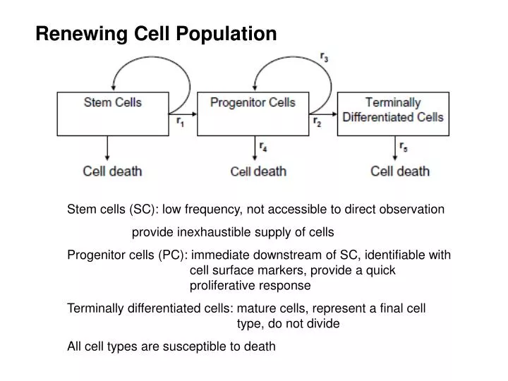
Stem cells (SC): low frequency, not accessible to direct observation

1. Renewing Cell Population Stem cells (SC): low frequency, not accessible to direct observation provide inexhaustible supply of cells Progenitor cells (PC): immediate downstream of SC, identifiable with cell surface markers, provide a quick proliferative response Terminally differentiated cells: mature cells, represent a final cell type, do not divide All cell types are susceptible to death

2. Example of renewing cell systems To: Stem cell T1: Glial-restricted precursor (GRP) T2: oligodendrocyte/type-2 astrocyte (O-2A)/oligodendrocyte precursor cell (OPC) (O-2A/OPC) • Development of Oligodendrocytes • Kinetics of Leukemic cells To: Leukemic stem cell (LSC) T1: Leukemic progenitor (LP) T2: Leukemic blast (LB)

3. Age-dependent Branching Process of Progenitor Cell Evolution without Immigration • Evolution of an individual PC from birth to leaving Every PC with probability p has a random life-time with probability 1 - p it differentiates into another cell type At the end of its life, every PC gives rise to v offsprings v characterized by pgf generally, it takes a random time for differentiation to occur

4. Stochastic processes Z(t), Z(t, x) Z(t) ~ total number of PCs Z(t, x) ~ number of PCs of note that if then, • pgfs of Z(t) , Z(t, x) • Applying the law of total probability (LTP)

5. Using notations: with initial conditions: • From (1) and (2): with initial conditions :

6. (3) is a renewal type equation with solution: where, and is the k-fold convolution renewal function

7. Renewal-type Non-homogeneous Immigration • Let Y(t) be the number of PCs at time t with the same evolution of Z(t) in the presence of immigration Y(t, x) number of PCs of • pgfs of Y(t) and Y(t, x) with initial conditions • time periods between the successive events of immigration: i.i.d, r.v.’s with c.d.f. at any given t, number of immigrants is random with distribution

8. pgf of number of immigrants at time t mean number of immigrants at time t • Applying LTP (10) (11) with initial conditions:

9. (12) (13) with initial conditions: • Whenever is bounded, (12) has a unique solution which is bounded on any finite interval • The solution is: where is the renewal function

10. Modeling of Neurogenesis Neurogenic Cascade d  apoptosis rate  rate of G2M in ANP2 differentiating into NB

11. The m matrix where mik is the expected number of progeny of type k at time t of a cell of type i dij is the probability of its corresponding type of cells committed to apoptosis, is the chance that cell differentiated to NB directly from the phase G2M in the process of ANP2

12. Model Construction We obtain the fundamental solution of the model where M is a matrix, with number of cells at time t in compartment j, given the population was seeded by a single cell in compartment i under physiological conditions, the system is fed by a stationary influx of freshly activated ANPs, which may be represented by a Poisson process with constant intensity ω per unit of time, thus we obtain

13. To calculate the stationary distribution of M we need to derive the inverse matrix of I-m The inverse of an upper triangular matrix is also an upper triangular matrix

15. Parameters in the inverse matrix are defined as

16. Example A computational example in simulating pulse labeling experiment with parameters T1=10 hr, T2=8 hr, T3=4 hr, T4=96 hr, T5=1hr, dij=0.15, α=0.5

17. Comparison suggests non-identical distribution of the mitotic cycle duration for amplifying neuroprogenitors (ANP) and unevenly distributed cell death rates