Download
1 / 15
150 likes | 322 Views
Data Dimensionality Reduction: Introduction to Principal Component Analysis Case Study: Multivariate Analysis of Chemistry-Property data in Molten Salts C. Suh 1 , S. Graduciz 2 , M. Gaune-Escard 2 , K. Rajan 1 Combinatorial Sciences and Materials Informatics Collaboratory

E N D
Data Dimensionality Reduction: Introduction to Principal Component Analysis Case Study: Multivariate Analysis of Chemistry-Property data in Molten Salts C. Suh1, S. Graduciz2, M. Gaune-Escard2 , K. Rajan1 Combinatorial Sciences and Materials Informatics Collaboratory 1 Iowa State University 2 CNRS , Marseilles, France
PRINCIPAL COMPONENT ANALYSIS: PCA From a set of N correlated descriptors, we can derive a set of N uncorrelated descriptors (the principal components). Each principal component (PC) is a suitable linear combination of all the original descriptors. PCA reduces the information dimensionality that is often needed from the vast arrays of data in a way so that there is minimal loss of information . ( from Nature Reviews Drug Discovery1, 882-894 (2002) : INTEGRATION OF VIRTUAL AND HIGH THROUGHPUT SCREENING Jürgen Bajorath ; and Materials Today; MATERIALS INFORMATICS , K. Rajan , October 2005
Functionality 1 = F ( x1 , x2 , x3 , x4 , x5 , x6 , x7 , x8 ……) Functionality 2 =F ( x1 , x2 , x3 , x4 , x5 , x6 , x7 , x8 ……) I ……. X1 = f ( x2) X2 = g( x3) X3= h(x4) PC 1= A1 X1 + A2 X2 + A3 X3 + A4 X4 ……. PC 2 = B1 X1 + B2 X2 + B3 X3 +B4 X4 ……. PC 3 = C1 X1 + C2 X2 + C3 X3 + C4 X4……. II III …….
DIMENSIONALITY REDUCTION: Case study • Database of molten salts properties tabulates numerous properties for each chemistry : • What can we learn beyond a “search and retrieve” function? • Can we find a multivariate correlation (s) among all chemistries and properties? • Challenge of reducing the dimensionality of the data set
Principal component analysis (PCA) involves a mathematical procedure that transforms a number of (possibly) correlated variables into a (smaller) number of uncorrelated variables called principal components. The first principal component accounts for as much of the variability in the data as possible, and each succeeding component accounts for as much of the remaining variability as possible.
Melting point = F ( x1 , x2 , x3 , x4 , x5 , x6 , x7 , x8 ……) Density =F ( x1 , x2 , x3 , x4 , x5 , x6 , x7 , x8 ……) Where xi = molten salt compound chemistries Dimensionality Reduction of Molten Salts Data (Janz’s Molten Salts Database:1700 chemistries with 7 variables.) …… X1 = f(x2) X2 = g(x3) X3= h(x4) …….
Mathematically, PCA relies on the fact that most of the descriptors are interrelated and these correlations in some instances are high. It results in a rotation of the coordinate system in such a way that the axes show a maximum of variation (covariance) along their directions. • This description can be mathematically condensed to a so-called eigenvalue problem. • The data manipulation involves decomposition of the data matrix X into two matrices T and P. The two matricesP and T are orthogonal. The matrix P is usually called the loadings matrix, and the matrix T is called the scores matrix. • The eigenvectors of the covariance matrix constitute the principal components. The corresponding eigenvalues give a hint to how much "information" is contained in the individual components.
The loadings can be understood as the weights for each original variable when calculating the principal component. The matrix Tcontains the original data in a rotated coordinate system. • The mathematical analysis involves finding these new “data” matrices T and P. The dimensions of T( ie its rank) that captures all the information of the entire data set of A ( ie # of variables) is far less than that of X ( ideally 2 or 3). One now compresses the N dimensional plot of the data matrix X into 2 or 3 dimensional plot of T and P.
PC 1= A1 X1 + A2 X2 + A3 X3 + A4 X4 ……. PC 2 = B1 X1 + B2 X2 + B3 X3 +B4 X4 ……. PC 3 = C1 X1 + C2 X2 + C3 X3 + C4 X4……. • The first principal component accounts for the maximum variance (eigenvalue) in the original dataset. The second, third ( and higher order) principal components are orthogonal (uncorrelated) to the first and accounts for most of the remaining variance. • A new row space is constructed in which to plot the data, where the axes represent the weighted linear combinations of the variables affecting the data. Each of these linear combinations are independent of each other and hence orthogonal. • The data when plotted in this new space is essentially a correlation plot, where the position of each data point not only captures all the influences of the variables on that data but also its relative influence compared to the other data.
Minimal contribution to additional information content beyond higher order principal components.. “Scree” plot helps to identify the # of PCs needed to capture reduced dimensionality NB…depending upon nature of data set, this can be within 2, 3 or higher principal components but still less than the # of variables in original data set Eigenvalue PC1 PC2 PC3 PC4 PC5 ……………
Thus the mth PC is orthogonal to all others and has the mth largest variance in the set of PCs. Once the N PCs have been calculated using eigenvalue/ eigenvector matrix operations, only PCs with variances above a critical level are retained (scree test). The M-dimensional principal component space has retained most of the information from the initial N-dimensional descriptor space, by projecting it into orthogonal axes of high variance. The complex tasks of prediction or classification are made easier in this compressed, reduced dimensional space.
Dimensionality Reduction of Molten Salts Data (Janz’s Molten Salts Database:1700 instances with 7 variables.) Multivariate (PCA) representation of the data sets Bivariate representation of the data sets
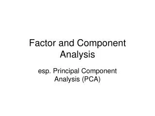
INTERPRETATIONS OF PRINCIPAL COMPONENT PROJECTIONS Correlations between variables captured in loading plot Trends in bonding capturedalong the PC1 axis of scoring plot
PCA : summary • To summarize, when we start with a multivariate data matrix PCA analysis permits us to reduce the dimensionality of that data set. This reduction in dimensionality now offers us better opportunities to: • Identify the strongest patterns in the data • Capture most of the variability of the data by a small fraction of the total set of dimensions • Eliminate much of the noise in the data making it beneficial for both data mining and other data analysis algorithms