Download
1 / 37
370 likes | 375 Views
CS61C Anatomy of I/O Devices: Magnetic Disks Lecture 15. March 10, 1999 Dave Patterson (http.cs.berkeley.edu/~patterson) www-inst.eecs.berkeley.edu/~cs61c/schedule.html. “Review..” 1/2. Protocol suites allow heterogeneous networking Another use of principle of abstraction

E N D
CS61CAnatomy of I/O Devices: Magnetic Disks Lecture 15 March 10, 1999 Dave Patterson (http.cs.berkeley.edu/~patterson) www-inst.eecs.berkeley.edu/~cs61c/schedule.html
“Review..” 1/2 • Protocol suites allow heterogeneous networking • Another use of principle of abstraction • Protocols operation in presence of failures • Standardization key for LAN, WAN • Integrated circuit revolutionizing network switches as well as processors • Switch just a specialized computer • High bandwidth networks with slow SW overheads don’t deliver their promise
Outline • Basic Terms/ Mechanical Operation • Disk Trends, State-of-the-Art, History • Disk Performance • Administrivia, “What’s this Stuff Good for” • Disk Fallacies (stump your OS prof!) • Disk Arrays, Reliability • RAID • Conclusion
Keyboard, Mouse Computer Processor (active) Devices Memory (passive) (where programs, data live when running) Input Disk, Network Control (“brain”) Output Datapath (“brawn”) Display, Printer Magnetic Disks • Purpose: • Long-term, nonvolatile, inexpensive storage for files • Large, inexpensive, slow level in the memory hierarchy (discuss later)
Inner Track Outer Track Sector Head Arm Platter Actuator Disk Device Terminology • Several platters, with information recorded magnetically on both surfaces (usually) • Bits recorded in tracks, which in turn divided into sectors (e.g., 512 Bytes) • Actuator moves head (end of arm,1/surface) over track (“seek”), select surface, wait for sector rotate under head, then read or write • “Cylinder”: all tracks under heads
{ Platters (12) Photo of Disk Head, Arm, Actuator Spindle Arm Head Actuator
Disk Device Performance Inner Track Outer Track Sector Head Controller Arm Spindle • Disk Latency = Seek Time + Rotation Time + Transfer Time + Controller Overhead • Seek Time? depends no. tracks move arm, seek speed of disk • Rotation Time? depends on speed disk rotates, how far sector is from head • Transfer Time? depends on data rate (bandwidth) of disk, size of request Platter Actuator
Disk Device Performance • Average distance sector from head? • 1/2 time of a rotation • 7200 Revolutions Per Minute 120 Rev/sec • 1 revolution = 1/120 sec 8.33 milliseconds • 1/2 rotation (revolution) 4.16 ms • Average no. tracks move arm? • Calculate all possible seek distances from all possible tracks • Answer: about 1/3 number of tracks • (Disk industry standard benchmark)
Data Rate: Inner vs. Outer Tracks • To keep things simple, orginally kept same number of sectors per track • Since outer track longer, lower bits per inch • Competition decided to keep BPI the same for all tracks (“constant bit density”) More capacity per disk More of sectors per track towards edge Since disk spins at constant speed, outer tracks have faster data rate • Bandwidth outer track 1.5X inner track!
State of the Art: Seagate Cheetah 36 • 36.4 GB, 3.5 inch disk • 12 platters, 24 surfaces • 10,000 RPM • 18.3 to 28 MB/s internal media transfer rate • 9772 cylinders (tracks), (71,132,960 sectors total) • Avg. seek: read 5.2 ms, write 6.0 ms (Max. seek: 12/13,1 track: 0.6/0.9 ms) • $2100 or 17MB/$ (6¢/MB) • 0.15 ms controller time Head Arm Track Sector Cylinder Platter Disk Controller Actuator source: www.seagate.com
Disk Performance Example • Calculate time to read 1 sector (512B) for Cheetah 36 using advertised performance; sector is on outer track Disk latency = average seek time + average rotational delay + transfer time + controller overhead = 5.2 ms + 0.5 * 1/(10000 RPM) + 0.5 KB / (28 MB/s) + 0.15 ms = 5.2 ms + 0.5 /(10000 RPM/(60000ms/M)) + 0.5 KB / (28 KB/ms) + 0.15 ms = 5.2 + 3.0 + 0.18 + 0.15 ms = 8.53 ms
Areal Density • Bits records along track • Metric is Bits Per Inch (BPI) • Number of tracks per surface • Metric is Tracks Per Inch (TPI) • Care about bit density per units area • Metric is Bits Per Square Inch • Called Areal Density • Areal Density =BPI x TPI
Disk History (IBM) Data density Mbit/sq. in. Capacity of Unit Shown Megabytes 1973: 1. 7 Mbit/sq. in 140 MBytes 1979: 7. 7 Mbit/sq. in 2,300 MBytes source: New York Times, 2/23/98, page C3, “Makers of disk drives crowd even more data into even smaller spaces”
Disk History 1989: 63 Mbit/sq. in 60,000 MBytes 1997: 1450 Mbit/sq. in 2300 MBytes 1997: 3090 Mbit/sq. in 8100 MBytes source: New York Times, 2/23/98, page C3, “Makers of disk drives crowd even more data into even smaller spaces”
Areal Density • Areal Density =BPI x TPI • Change slope 30%/yr to 60%/yr about 1991
Historical Perspective • Form factor plus capacity drives market, not so much performance • 1970s: Mainframes 14 inch diameter disks • 1980s: Minicomputers, Servers 8”, 5.25” diameter disks • Late 1980s/Early 1990s: • Pizzabox PCs 3.5 inch diameter disks • Laptops, notebooks 2.5 inch disks • Palmtops didn’t use disks, so 1.8 inch diameter disks didn’t make it
1 inch disk drive! • 1999 IBM MicroDrive: • 1.7” x 1.4” x 0.2” • 340 MB, 5400 RPM, 5 MB/s, 15 ms seek • Digital camera, PalmPC? • 2006 MicroDrive? • 9 GB, 50 MB/s! • Assuming it finds a niche in a successful product • Assuming past trends continue
Administrivia • 6th homework: Due Today (8AM tomorrow) • 4th Project: Friday 3/12 7PM(absolute latest: 3/13 8AM) • Readings: Cache Memory 7.1, 7.2 • Upcoming events • Midterm Review Sunday 3/14 2PM, 1 Pimentel • Midterm on Wed. 3/17 5pm-8PM, 1 Pimentel • Friday before Break 3/19: video tape by Gordon Moore, “Nanometers and Gigabucks” • Copies of lecture slides in 271 Soda? Copies before midterm in Copy Central? $10
“What’s This Stuff Good For?” Computers with wireless modems let drivers keep in touch with headquarters through E-mail. Companies can send out fleetwide communications, and drivers can tell dispatchers about any delays. A truck using this Global Positioning System (GPS) technology sends signals to satellites, which send the truck's position to system's manufacturer, Qualcomm. That information is relayed to trucking company dispatchers. Collision-avoidance systems based on radar make alarms go off if a truck gets too close to another vehicle, giving the driver time to take evasive action. Such systems can also track whether a driver habitually tailgates and pass that information along to the company. N.Y. Times, 3/4/99
Fallacy: Use Data Sheet “Average Seek” Time • Manufacturers needed standard for fair comparison (“benchmark”) • Calculate all seeks from all tracks, divide by number of seeks = “average” • Real average would be based on how data laid out on disk, where seek in real applications, then measure performance • Usually, tend to seek to tracks nearby, not to random track • Rule of Thumb: observed average seek time is typically about 1/4 to 1/3 of quoted seek time (i.e., 3X-4X faster) • Cheetah 36 avg. seek: 5.2 ms 1.7 ms
Fallacy: Use Data Sheet Transfer Rate • Manufacturers quote the speed off the data rate off the surface of the disk • Sectors contain an error detection and correction field (can be 20% of sector size) plus sector number as well as data • There are gaps between sectors on track • Rule of Thumb: disks deliver about 3/4 of internal media rate (1.3X slower) for data • For example, Cheetah 36 quotes 28 to 18 MB/s internal media rate Expect 21 to 14 MB/s user data rate
Disk Performance Example • Calculate time to read 1 sector for Cheetah 36 again, this time using 1/3 quoted seek time, 3/4 of internal outer track bandwidth; (8.53 ms before) Disk latency = average seek time + average rotational delay + transfer time + controller overhead = (0.33 * 5.2 ms) + 0.5 * 1/(10000 RPM) + 0.5 KB / (0.75 * 28 MB/s) + 0.15 ms = 1.73 ms + 0.5 /(10000 RPM/(60000ms/M)) + 0.5 KB / (21 KB/ms) + 0.15 ms = 1.73 + 3.0 + 0.24 + 0.15 ms = 4.73 ms
Disk Performance Model /Trends • Capacity + 60%/year (2X / 1.5 yrs) • Transfer rate (BW) + 40%/year (2X / 2.0 yrs) • Rotation + Seek time – 8%/ year (1/2 in 10 yrs) • MB/$ > 60%/year (2X / <1.5 yrs) Fewer chips + areal density
Future Disk Size and Performance • Continued advance in capacity (60%/yr) and bandwidth (40%/yr) • Slow improvement in seek, rotation (8%/yr) • Time to read whole disk Year Sequentially Randomly (1 sector/seek) 1990 4 minutes 6 hours 2000 12 minutes 1 week(!) • 3.5” form factor make sense in 5-7 yrs?
Use Arrays of Small Disks? • Randy Katz and myself asked in 1987: • Can smaller disks be used to close gap in performance between disks and CPUs? Conventional: 4 disk designs 3.5” 5.25” 10” 14” High End Low End Disk Array: 1 disk design 3.5”
Replace Small Number of Large Disks with Large Number of Small Disks! (1988 Disks) IBM 3390K 20 GBytes 97 cu. ft. 3 KW 15 MB/s 600 I/Os/s 250 KHrs $250K x70 23 GBytes 11 cu. ft. 1 KW 120 MB/s 3900 IOs/s ??? Hrs $150K IBM 3.5" 0061 320 MBytes 0.1 cu. ft. 11 W 1.5 MB/s 55 I/Os/s 50 KHrs $2K Capacity Volume Power Data Rate I/O Rate MTTF Cost Disk Arrays have potential for large data and I/O rates, high MB per cu. ft., high MB per KW, but what about reliability?
Array Reliability • Reliability - whether or not a component has failed • measured as Mean Time To Failure (MTTF) • Reliability of N disks = Reliability of 1 Disk ÷ N • 50,000 Hours ÷ 70 disks = 700 hour • Disk system MTTF: Drops from 6 years to 1 month! • Arrays too unreliable to be useful!
Redundant Arrays of (Inexpensive) Disks • Files are "striped" across multiple disks • Redundancy yields high data availability • Availability: service still provided to user, even if some components failed • Disks will still fail • Contents reconstructed from data redundantly stored in the array Capacity penalty to store redundant info Bandwidth penalty to update redundant info
Redundant Arrays of Inexpensive DisksRAID 1: Disk Mirroring/Shadowing recovery group • • Each disk is fully duplicated onto its “mirror” • Very high availability can be achieved • • Bandwidth sacrifice on write: • Logical write = two physical writes • • Reads may be optimized • • Most expensive solution: 100% capacity overhead • (RAID 2 not interesting, so skip)
10010011 11001101 10010011 . . . P 1 0 0 1 0 0 1 1 1 1 0 0 1 1 0 1 1 0 0 1 0 0 1 1 1 1 0 0 1 1 0 1 logical record Striped physical records Redundant Array of Inexpensive Disks RAID 3: Parity Disk P contains sum of other disks per stripe mod 2 (“parity”) If disk fails, subtract P from sum of other disks to find missing information
RAID 3 • Sum computed across recovery group to protect against hard disk failures, stored in P disk • Arms logically synchronized • Logically, a single high capacity, high transfer rate disk: good for large transfers • Wider arrays reduce capacity costs, but decreases availability • 33% capacity cost for parity in this configuration
Inspiration for RAID 4 • RAID 3 relies on parity disk to discover errors on Read • But every sector has an error detection field • Rely on error detection field to catch errors on read, not on the parity disk • Allows independent reads to different disks simultaneously
Stripe Redundant Arrays of Inexpensive Disks RAID 4: High I/O Rate Parity Increasing Logical Disk Address D0 D1 D2 D3 P Insides of 5 disks D7 P D4 D5 D6 D8 D9 D10 P D11 Example: small read D0 & D5, large write D12-D15 D12 D13 P D14 D15 D16 D17 D18 D19 P D20 D21 D22 D23 P . . . . . . . . . . . . . . . Disk Columns
D0 D1 D2 D3 P D7 P D4 D5 D6 Inspiration for RAID 5 • RAID 4 works well for small reads • Small writes (write to one disk): • Option 1: read other data disks, create new sum and write to Parity Disk • Option 2: since P has old sum, compare old data to new data, add the difference to P • Small writes are limited by Parity Disk: Write to D0, D5 both also write to P disk
Redundant Arrays of Inexpensive Disks RAID 5: High I/O Rate Interleaved Parity Increasing Logical Disk Addresses D0 D1 D2 D3 P Independent writes possible because of interleaved parity D4 D5 D6 P D7 D8 D9 P D10 D11 D12 P D13 D14 D15 Example: write to D0, D5 uses disks 0, 1, 3, 4 P D16 D17 D18 D19 D20 D21 D22 D23 P . . . . . . . . . . . . . . . Disk Columns
Berkeley History: RAID-I • RAID-I (1989) • Consisted of a Sun 4/280 workstation with 128 MB of DRAM, four dual-string SCSI controllers, 28 5.25-inch SCSI disks and specialized disk striping software • Today RAID is multi billion dollar industry, > 50 companies, from PCs to mainframes; mainly availability
“And in Conclusion..” 1/1 • Magnetic Disks continue rapid advance: 60%/yr capacity, 40%/yr bandwidth, slow on seek, rotation improvements, MB/$ improving 100%/yr? • Designs to fit high volume form factor • Quoted seek times too conservative, data rates too optimistic for use in system • RAID • Higher performance with more disk arms per $ • Adds availability option at modest cost • Next: Introduction to Memory Hierarchy, Review of 1st 8 weeks of 61C