Download
1 / 56
590 likes | 651 Views
Feature Selection. Machine Learning Workshop August 23 rd , 2007 Alex Shyr. Adapted from Ben Blum’s Slides. Outline. Introduction What is feature selection? Why do it? Filtering Model selection Model evaluation Model search Regularization Kernel methods Miscellaneous topics Summary.

E N D
Feature Selection Machine Learning Workshop August 23rd, 2007 Alex Shyr Adapted from Ben Blum’s Slides
Outline • Introduction • What is feature selection? Why do it? • Filtering • Model selection • Model evaluation • Model search • Regularization • Kernel methods • Miscellaneous topics • Summary
Introduction • Data: pairs • : vector of features • Features can be real ( ), categorical ( ), or more structured • y: response (dependent) variable • : binary classification • : regression • Typically, this is what we want to be able to predict, having observed some new .
Featurization • Data is often not originally in vector form • Have to choose features • Features often encode expert knowledge of the domain • Can have a huge effect on performance • Example: documents • “Bag of words” featurization: throw out order, keep count of how many times each word appears. • Surprisingly effective for many tasks
What is feature selection? • Reducing the feature space by throwing out some of the features (covariates) • Also called variable selection • Motivating idea: try to find a simple, “parsimonious” model • Occam’s razor: simplest explanation that accounts for the data is best • Augmenting feature space to fit better model • see kernel methods
What is feature selection? Task: classify whether a document is about cats Data: word counts in the document X Reduced X
Why do it? • Case 1 (Interpretation): • We’re interested in features—we want to know which are relevant. The model should be interpretable. • Case 2 (Performance): • We’re interested in prediction; we just want to build a good predictor, with as little features as possible. • By removing redundant and irrelevant features, we can usually improve model performance. • By adding to and enriching the feature space, we can also improve model performance.
Why do it? Case 1. We want to know which features are relevant. Examples • What causes lung cancer? • Features are aspects of a patient’s medical history • Binary response variable: did the patient develop lung cancer? • Which features best predict whether lung cancer will develop? Might want to legislate against these features. • What causes a program to crash? [Alice Zheng ’03, ’04, ‘05] • Features are aspects of a single program execution • Which branches were taken? • What values did functions return? • Binary response variable: did the program crash? • Features that predict crashes well are probably bugs.
Why do it? Case 2. We want to build a good predictor. Examples • Text classification • Features for all 105 English words, and maybe all word pairs • Common practice: throw in every feature you can think of, let feature selection get rid of useless ones • Training too expensive with all features • The presence of irrelevant features hurts generalization. • Embedded systems with limited resources • Voice recognition on a cell phone • Branch prediction in a CPU (4K code limit) • Classifier must be compact
Outline • Review/introduction • What is feature selection? Why do it? • Filtering • Model selection • Model evaluation • Model search • Regularization • Kernel methods • Miscellaneous topics • Summary
Filtering • Simple techniques for weeding out irrelevant features without fitting model
Filtering • Basic idea: assign score to each feature indicating how “related” and are. • Intuition: if for all i, then feature is good no matter what our model is—contains all information about . • Many popular scores [see Yang and Pederson ’97] • Classification with categorical data: Chi-squared, information gain • Can use binning to make continuous data categorical • Regression: correlation, mutual information • Markov blanket [Koller and Sahami, ’96] • Then somehow pick how many of the highest scoring features to keep (nested models)
Comparison of filtering methods for text categorization [Yang and Pederson ’97]
Filtering • Advantages: • Very fast • Simple to apply • Disadvantages: • Doesn’t take into account which learning algorithm will be used. • Doesn’t take into account correlations between features • This can be an advantage if we’re only interested in ranking the relevance of features, rather than performing prediction. • Suggestion: use light filtering as an efficient initial step if there are many obviously irrelevant features • Caveat here too—apparently useless features can be useful when grouped with others
Outline • Introduction • What is feature selection? Why do it? • Filtering • Model selection • Model evaluation • Model search • Regularization • Kernel methods • Miscellaneous topics • Summary
Model Selection • Choosing between possible models of varying complexity • In our case, a “model” means a set of features • Running example: linear regression model
Linear Regression Model Model Prediction rule: Data Response: Parameters • Typical loss function is sum squared error: • Recall that we can fit it via the normal equations: • Can be interpreted as maximum likelihood with
Model Selection Model Prediction rule: Data Response: Parameters • Consider a reduced model with only those features for • Squared error is now • We want to pick out the “best” . Maybe this means theone with the lowest training error ? • Note • Just zero out terms in to match . • Generally speaking, training error will only go up in a simpler model. So why should we use one?
30 25 Degree 15 polynomial 20 15 10 5 0 -5 -10 -15 0 2 4 6 8 10 12 14 16 20 18 Overfitting example • This model is too rich for the data • Fits training data well, but doesn’t generalize.
Model evaluation • Moral 1: In the presence of many irrelevant features, we might just fit noise. • Moral 2: Training error can lead us astray. • To evaluate a feature set , we need a better scoring function • We’ve seen that is not appropriate. • We’re not ultimately interested in training error; we’re interested in test error (error on new data). • We can estimate test error by pretending we haven’t seen some of our data. • Keep some data aside as a validation set.
K-fold cross validation • A technique for estimating test error • Uses all of the data to validate • Divide data into K groups . • Use each group as a validation set, then average all validation errors X7 X1 X6 test Learn X2 X5 X3 X4
K-fold cross validation • A technique for estimating test error • Uses all of the data to validate • Divide data into K groups . • Use each group as a validation set, then average all validation errors X7 X1 X6 Learn X2 test X5 X3 X4
K-fold cross validation • A technique for estimating test error • Uses all of the data to validate • Divide data into K groups . • Use each group as a validation set, then average all validation errors X7 X1 X6 Learn X2 X5 X3 X4
Model Search • We have an objective function • Time to search for a good model. • This is known as a “wrapper” method • Learning algorithm is a black box • Just use it to compute objective function, then do search • Exhaustive search expensive • 2n possible subsets • Greedy search is common and effective
Model search Forward selection Initialize s={} Do: Add feature to s which improves K(s) most While K(s) can be improved Backward elimination Initialize s={1,2,…,n} Do: remove feature from s which improves K(s) most While K(s) can be improved • Backward elimination tends to find better models • Better at finding models with interacting features • But it is frequently too expensive to fit the large models at the beginning of search • Both can be too greedy.
Model search • More sophisticated search strategies exist • Best-first search • Stochastic search • See “Wrappers for Feature Subset Selection”, Kohavi and John 1997 • For many models, search moves can be evaluated quickly without refitting • E.g. linear regression model: add feature that has most covariance with current residuals • YALE can do feature selection with cross-validation and either forward selection or backwards elimination. • Other objective functions exist which add a model-complexity penalty to the training error • AIC: add penalty to log-likelihood. • BIC: add penalty
Outline • Review/introduction • What is feature selection? Why do it? • Filtering • Model selection • Model evaluation • Model search • Regularization • Kernel methods • Miscellaneous topics • Summary
Regularization • In certain cases, we can move model selection into the induction algorithm • Only have to fit one model; more efficient. • This is sometimes called an embedded feature selection algorithm
Regularization • Regularization: add model complexity penalty to training error. • for some constant C • Now • Regularization forces weights to be small, but does it force weights to be exactly zero? • is equivalent to removing feature f from the model
L1 vs L2 regularization • To minimize , we can solve by (e.g.) gradient descent. • Minimization is a tug-of-war between the two terms
L1 vs L2 regularization • To minimize , we can solve by (e.g.) gradient descent. • For L1 regularization, w is forced into the corners • many components 0 • Solution is sparse
L1 vs L2 regularization • To minimize , we can solve by (e.g.) gradient descent. • L2 regularization does not promote sparsity • Even without sparsity, regularization promotes generalization • limits expressiveness of model
Lasso Regression [Tibshirani ‘94] • Simply linear regression with an L1 penalty for sparsity. • Two big questions: • 1. How do we perform this minimization? • With L2 penalty it’s easy • With L1 it’s not a least-squares problem any more • 2. How do we choose C?
Least-Angle Regression • Up until a few years ago this was not trivial • Must fit model for every candidate C value • LARS (Least Angle Regression, Hastie et al, 2004) • Find trajectory of w for all possible C values simultaneously, as efficiently as least-squares • Can choose how many features are wanted Figure taken from Hastie et al (2004)
Outline • Review/introduction • What is feature selection? Why do it? • Filtering • Model selection • Model evaluation • Model search • Regularization • Kernel methods • Miscellaneous topics • Summary
Kernel Methods • Expanding feature space gives us new potentially useful features. • Kernel methods let us work implicitly in a high-dimensional feature space. • All calculations performed quickly in low-dimensional space.
Feature engineering • Linear models: convenient, fairly broad, but limited • We can increase the expressiveness of linear models by expanding the feature space. • E.g. • Now feature space is R6 rather than R2 • Example linear predictor in these features:
The kernel trick • Can still fit by old methods, but it’s more expensive • Many algorithms we’ve looked at only see data through inner products (or can be rephrased to do so) • Perceptron, logistic regression, etc. • But notice: • We can just compute inner product in original space. • This is called the kernel trick: • Working in high-dimensional feature space implicitly through an efficiently-computable inner product kernel.
Kernel methods • For some models, can write the coefficients as a linear combination of the data points • Update rule for perceptron: • Representer theorem: for many kinds of models with linear parameters w, we can write for some a. • For linear regression, our predictor can be written • Never need to deal with w explicitly; just need a kernel to take the place of in comparing data points to each other.
Kernel methods • Often more natural to define a similarity kernel than to define a feature space • Mercer theorem: every “qualifying” inner product kernel has an associated (possibly infinite-dimensional) feature space. • Polynomial kernels: • : feature space = all monomials in x and z of degree <= • RBF kernel: • : feature space is infinite dimensional
Dynamic programming string kernel[Lodhi et al, 2002] • Feature space: all possible substrings of k letters, not necessarily contiguous. • E.g. a-p-l-s in “apples are tasty” • Value for each feature is exp{-(full length of substring in text)} • Very high dimensional! • Surprisingly, kernel can be computed efficiently using dynamic programming. • Runs in time linear in length of documents • Text classification results: superior to using bag-of-words feature space. • No way we could use this feature space without kernel methods.
Kernel methods vs feature selection • Kernelizing is often, but not always, a good idea. • Often more natural to define a similarity kernel than to define a feature space, particularly for structured data • Sparsity • Typically regularize the model parameters • L1 norm gives sparse solutions • Solutions are sparse in the sense that only a few data points have non-zero weight: “support vectors”. • Feature/data exchange • After kernelization, data points act as features. • If many more (implicit) features than data points, more efficient • Given a set of support vectors , a new data point X has implicit feature vector • Prediction is then
Outline • Review/introduction • What is feature selection? Why do it? • Filtering • Model selection • Model evaluation • Model search • Regularization • Kernel methods • Miscellaneous topics • Summary
Decision Trees • Effectively a stepwise filtering method • In each subtree, only a subset of the data is considered • Split on top feature according to filtering criterion • Stop according to some stopping criterion • Depth, homogeneity, etc • In final tree, only a subset of features are used • Very useful with boosting • Connection between Adaboost and forward selection Tor23 A B Tor4 Tor27 A G B Tor4 Tor40 -130.2
Dimension Reduction • Principal Component Analysis (PCA) • Project onto subspace withthe most variance • Unsupervised learning(doesn’t take response y into account) • Sufficient Dimension Reduction • Project onto subspace where, given the projected data, the response is most independent from the data • Other dimensionality reduction techniques in future lecture
Outline • Review/introduction • What is feature selection? Why do it? • Filtering • Model selection • Model evaluation • Model search • Regularization • Kernel methods • Miscellaneous topics • Summary
Summary Computational cost • Filtering • L1 regularization (embedded methods) • Kernel methods • Wrappers • Forward selection • Backward selection • Other search • Exhaustive
Summary Computational cost • Filtering • L1 regularization (embedded methods) • Kernel methods • Wrappers • Forward selection • Backward selection • Other search • Exhaustive • Good preprocessing step • Information-based scores seem most effective • Information gain • More expensive: Markov Blanket [Koller & Sahami, ’97] • Fail to capture relationship between features
Summary Computational cost • Filtering • L1 regularization (embedded methods) • Kernel methods • Wrappers • Forward selection • Backward selection • Other search • Exhaustive • Fairly efficient • LARS-type algorithms now exist for many linear models • Not applicable for all models • Linear methods can be limited • Common: fit a linear model initially to select features, then fit a nonlinear model with new feature set