Download
1 / 31
310 likes | 314 Views
This study aims to examine the causal effect of hospice care on healthcare expenditures of nursing home residents at the end of life. It controls for selection bias and differences in costs due to informative attrition. Data from Florida in 1999 is used to analyze expenditures, utilization, and resident and facility characteristics.

E N D
The Effects of Hospice Care on Costs at the End-of-Life* Orna Intrator with Pedro Gozalo and Susan Miller Brown University * Funded by: AHRQ #HS10549
Background • Prior cost studies criticized for selection biases: • Patients electing hospice are potentially different • Nursing home residents can only elect hospice if nursing Home has contract with hospice provider • Select retrospective sample of patients who died
Study Aims • Study the causal effect of hospice on health care expenditures of nursing home residents. • Control for selection bias of patients and nursing home facilities. • Control for differences in costs due to informative attrition due to survival differentials among patients.
Hospice Selection • Hospice treatment is not randomly assigned (selection bias potential). • Hospice is both an outcome of health and a predictor of costs. • In other words: hospice selection is an endogenous process to both mortality and expenditures. • ORDINARY REGRESSION MODELS WILL PROVIDE BIASED CAUSAL EFFECT ESTIMATES (Jamie Robins and others)
Informative Censoring • Residents who are more likely to die are more likely to choose hospice • Residents who are more likely to die are more likely to accumulate higher expenditures • Survival process is endogenous to both hospice and expenditure processes
Data Sources (Florida,1999) • Expenditures and utilization: • Medicare eligibility (denominator) and claims (SAF): inpatient, skilled nursing services (SNF), hospice, home health, outpatient • Medicaid buckets • Resident nursing home assessment data (MDS RAI) • Nursing homes: Online Survey Certification Automated Records (OSCAR)
Medicare & Medicaid Expenditure Data • Aggregate all expenditure categories • Average daily expenditures in period • Period usually 1 week (96%) • Period shorter in week of death • Daily periods during week of transition to hospice (2.8%) • Prospective data for 6 months in periods
Healthcare Utilization Data • In each period • Hospital days • Hospice days in nursing home • Hospice days in hospital • Medicare skilled services days (SNF) • Prior 3 months utilization/expenditure history • Hospitalizations • SNF use • Home health care use • Total prior expenditures
Resident and Facility Data • Clinical data from nursing home assessments (MDS) at baseline: • Demographics • Diagnoses, conditions, medications • Advance directives (care preferences) • Nursing home data from OSCAR: • Organizational structure (profit, chain, size) • Staffing • Available services • Resident casemix severity
Cohort Selection • Nursing home residents in Florida with MDS assessment in 4-6/1999 • No prior hospice • Hospice eligible • Upper quartile of predicted probability: • Predicted Pr(Death in 6 months) > 0.2 • For data completeness: • Age 65+ • No HMO throughout 1999 • Dual Medicare-Medicaid eligible
Data Summary • During time interval (t-1,t] resident i in nursing home j accumulates expenditures Xjit . • Let: • Yjit = sqrt(Xjit) square-root expenditures • Cjit = I(died in time interval) • Hjit = I(hospice in time interval) • Covariates Zjit = (Ujit, Vji, Wi)
Joint Modeling Approach • Endogenous processes in time • Model joint distribution (Y,C,H)jit • Joint underlying frailty • Follows Lancaster & Intrator (JASA, 1998) • Estimation requires MCMC methods
Model Simplification • Given covariates Zjit model: • E(Yjit |hjit, cjit, zjit) • Yjit is average expenditure in period • May depend on time since hospice selection • GEE methods to account for repeat observation per resident, and per facility • Distributional assumptions about Y are not required • The within-patient correlation matrix does not have to be correctly specified.
Adjusting for Selection • Informative attrition is considered another selection process • E(Hjit, Cjit) = E(Hjit | cjit) E(Cjit) • Inverse probability weighting using propensity scores • Potentially better control for unobserved confounders • Use time-specific weights • Stabilized by using ratio of time-specific propensity to overall or resident-specific propensity
Survival and Hospice Selection Model Estimation • Assume hospice selection is “terminal” • Markovian data structure for repeat observation of survival and hospice selection • Assume independent periods within resident • Adjust for within-nursing home correlation
Estimation of Weights • Estimate intensities of hospice selection and mortality at each time period • Logit Pr(Hjit | cjit=0, Zjit-1) • Logit Pr(Cjit=1 | Zjit-1, Hjit) • Kaplan-Meier estimates of propensity scores • Stabilize inverse weights • Combine weights: • E(Hjit, Cjit) = E(Hjit | cjit) E(Cjit)
Results • Separate analyses for Short (<90 days) and Long Stay (90+ days) NH residents • Separate analyses by Main Diagnostic group: • Cancer • No Cancer, any dementia • Other
“Other” Diagnoses Cohorts Long Stay • 62,591 periods • 2,846 residents • 564 facilities • 228 residents with hospice in 167 facilities • 793 (28%) died • Median hospice LOS = 19days Short Stay • 53,525 periods • 2,474 residents • 588 facilities • 161 residents with hospice in 129 facilities • 588 (24%) died • Median hospice LOS = 19days
Short Stay with Dx=“Other” Multivariate Average Daily Total Expenditures
Long Stay with Dx=“Other” Multivariate Average Daily Total Expenditures
Summary • Controlling for hospice selection and attrition is important. • Biggest hospice effect for Short-Stay NH residents: SAVINGS in first 3 weeks and no significant difference afterwards. • Long-stay resident have HIGHER EXPENSES after the 3rd week in hospice.
Limitations • Effects on “intensity” of costs, not total costs. • How to draw inference regarding effects on total costs? • Hospice selection estimated only on residents in NHs offering hospice (82% in Florida): • May not adequate for other states. • Results are not of a joint model • potential for effects on costs to be confounded with effects on death
FIN Thank you for your attention! Comments welcome… Orna_Intrator@Brown.Edu
Extensions • Generalize hospice choice model • Interaction between nursing home and hospice providers in hospice contracting • Estimate joint model of end-of-life expenditures, with hospice selection and survival censoring. • Examine cost-effectiveness of hospice using quality of end-of-life measure
Comparison with Retrospective Study • Retrospective model of hospice effect on expenditures in last month of life • Florida NH residents • Died in NH 7-12/1999 • Hospice savings effect was greater for short-stay NH residents • Difference in effect of residents with short/long time in hospice • Prospective model provides better control for LOS in hospice
Outline • Data and cohort selection • Model and Model simplification • Estimation • Results • Discussion
Inverse Probability-of-Treatment Weighting (IPTW) • Alternative to Propensity Score Matching or Stratification • Potentially better control for unobserved confounders • Use time-specific weights • Stabilized by using ratio of time-specific propensity to overall or resident-specific propensity
Inverse Probability Weights • Stabilized inverse probability weight for resident j in facility i at time t, product of: • stabilized survival weight S* • Stabilized hospice selection weight S • Stabilized weights based on estimation of propensities on subset L of covariates Z • We used overall probabilities of hospice selection and mortality • Use predicted probabilities. • Example: S* Pr(C=1|L)*Dead + Pr(C=0|L)*Alive Pr(C=1|Z)*Dead + Pr(C=0|Z)*Alive
Simulations for prediction: • E(Y|T=x, H=k, z) • Expected costs for persons surviving for x time period (weeks), and with hospice for k time period. • E(Y|t-s>0) / E(Y|t-s=0) • Ratio of total average additional costs of having any hospice versus having no hospice.