Download
1 / 40
400 likes | 410 Views
SPX and VIX: A Copula Approach. Kuan-Pin Lin Copula Seminar, February 23, 2006. SPX and VIX. SPX: Standard And Pool’s 500 Stock Index VIX: Implied Volatility Index Daily Time Series: 1990.1.2 to 2004.12.31 Questions: Are They Correlated? How? Is There Tail Dependence?

E N D
SPX and VIX: A Copula Approach Kuan-Pin Lin Copula Seminar, February 23, 2006
SPX and VIX • SPX: Standard And Pool’s 500 Stock Index • VIX: Implied Volatility Index • Daily Time Series: 1990.1.2 to 2004.12.31 • Questions: • Are They Correlated? How? • Is There Tail Dependence? • Does the Dependence Time-Varying?
Notations • SPX ln(SPX) R y v [0,1] • VIX ln(VIX) V x u [0,1]
SPX • SPX is the Standard and Pool’s 500 Index. It represents 70% of U.S. publicly traded companies listed on NYSE. The index is an average of the share prices weighted by the company’s market capitalization.
VIX • VIX is the Chicago Board of Trades index for implied volatility. It is calculated based on the daily at-the-money prices in both current and future contract periods. VIX or implied volatility is not about stock price swings, but about the associated option swings.
ln(SPX) and R = 100*ln(SPX/SPX-1) • ln(SPX) is non-stationary. • R = 100*ln(SPX/SPX-1), the rate of returns. • R is stationary.
ln(VIX) and V = 100*ln(VIX/VIX-1) • ln(VIX) is non-stationary (although VIX is stationary). • V = 100*ln(VIX/VIX-1), the rate of volatility change. • V is stationary.
R V N 3783 3783 Min -7.1127 -27.5054 Max 5.5732 41.6861 Mean 0.03211 -0.0068787 Variance 1.0669 31.287 Skewness -0.10457 0.59738 Kurtosis 6.6703 6.6398 R and V are Stationary but Non-Normal
The Univariate Time Series Model Let Y be either R or V. Conditional Mean Equation--AR(p): Yt = b0 + bZt + r1Yt-1 + …+ rpYt-p + et et = stut, where ut ~ nid(0,1) Conditional Variance Equation—Asymmetric GARCH(1,1): st2 = g0 + gZt + d1st-12 + (de+ daDt-1) et-12 Dt = asymmetry = 1 if et<0; 0 otherwise. Zt is the exogenous quantitative or qualitative variable(s). In this study, Zt = [Zt1, Zt2] where Zt1 = shift = 1 if t > 1997.6.30; 0 otherwise. Zt2 = trend = (t-1997.6.30)/(2004.12.31-1997.7.1) if t > 1997.6.30; 0 otherwise.
Quasi-Maximum-Likelihood Estimation Define ut = et/st. Log-likelihood function: t=1,2,…,Nln[f(ut)/st] ll(q) = – ½ N ln(2p) - ½ t=1,2,…,Nln(st2) –½ t=1,2,…,N (et2/st2) Quasi-Maximum-Likelihood Estimation is robust with respect to the potential model misspecification due to non-normality in the data: q* = (b,r,g,d) = maxarg q {ll(q)}
R V N 3783 3783 Conditional Mean Equation b0 -0.0040518 (0.011179) 0.37292 (0.064692) b1 Shift -0.39417 (0.089330) r1 -0.091304 (0.014548) r2 -0.069240 (0.014402) r3 -0.092740 (0.014991) r4 -0.072908 (0.014570) r5 -0.048615 (0.014480) r6 -0.087393 (0.013876) r7 -0.045888 (0.012269) -0.059696 (0.014356) r8 -0.044272 (0.014092) r11 -0.090808 (0.014007) r12 0.047202 (0.011774) Conditional Variance Equation g0 0.072265 (0.011100) 8.9837 (1.7231) g1 Shift 0.11154 (0.017014) -1.6184 (0.56658) g2 Trend -0.13992 (0.019960) -3.8370 (1.0113) d1 0.87859 (0.015402) 0.78062 (0.042170) de 0.0074855 (0.0065131) 0.15267 (0.026247) da Asymmetry 0.20212 (0.022551) -0.12735 (0.023865) Log-likelihood -6915.6 -9789.4 QML Estimates of Model Parameters Note: Numbers in parentheses are estimated standard errors.
Summary of Univariate Analysis I • There is 2-3 week or 12-day autocorrelation in the mean, for both R and V. • V has shifted down in the mean since 1997.7. • The mean of R has not changed.
Summary of Univariate Analysis II • There are persistence and asymmetry in the variance, for both R and V. • V has negative asymmetry in the variance, while R has positive asymmetry. • Both variances have shifted since 1997.7. For R, it has shifted upward, while the variance of V has shifted down. • Negative trend since 1997.7 in the variance is found for both R and V.
R V N 3771 3771 Min -7.1431 -22.762 Max 5.6179 40.279 Mean 0.037887 -0.25852 Variance 1.0616 30.1526 Skewness -0.10551 0.71943 Kurtosis 6.7016 6.6016 QML Residual Analysis Note: First 12 observations are deleted due to 12 lags used in the model estimation.
Standardized Residuals (Shocks) [yt] = QML estimates of (et/st) for R (top) [xt] = QML estimates of (et/st) for V (bottom)
y x N 3771 3771 Min -4.4787 -2.7928 Max 3.0657 6.1353 Mean 0.029033 -0.041349 Variance 0.58414 0.67322 Skewness -0.25272 0.62969 Kurtosis 4.2856 5.6791 Box-Pierce Test for ARMA Q1 1.7974 (0.18003) 1.4037 (0.23611) Q5 7.6692 (0.17543) 3.4198 (0.63556) Q10 8.6022 (0.57023) 5.1606 (0.88019) Q15 13.840 (0.53770) 8.0135 (0.92324) Box-Pierce Test for GARCH Q1 2.7150 (0.09941) 0.011653 (0.91404) Q5 8.8391 (0.11566) 2.2517 (0.81333) Q10 10.923 (0.36355) 11.741 (0.30276) Q15 15.488 (0.41687) 15.304 (0.42975) Kolmogorov-Smirnov Test Uniform 0.0003 0.0003 Normal 0.0432 0.0394 [y] and [x] Numbers in parentheses are p-values. K-S test critical values (N=3771): 10%, 0.019892651; 5%, 0.022070442; 1% 0.026458526
Summary of Univariate Analysis II • Standardized residuals y and x are i.i.d. • They are non-normal. • They are uniformly distributed. • Ready for copula-based correlation analysis.
Scatter Plot of (x,y): x on horizontal and y on vertical axis
Scatter Plot of (u,v): u=FX(x) on horizontal and v=FY(y) on vertical axis
N= 3771 c = -0.67468 t = -0.47510 r = -0.64935 Unconditional Correlations of (y,x) • Pearson = c • Kendall = t • Spearman = r
Unconditional Correlations of (y,x) • y (SPX shocks) and x (VIX shocks) are negatively correlated. • Is there a tail dependency?
N= 1411 c = -0.413 t = -0.246 r = -0.362 N= 474 c = 0.176 t = 0.008 r = 0.010 N= 474 c = -0.017 t = -0.035 r = -0.052 N= 1411 c = -0.639 t = -0.374 r = -0.530
N = 524 c = -0.339 t = -0.206 r = -0.305 N = 419 c = 0.196 t = 0.029 r = 0.030 N = 278 c = -0.069 t = -0.031 r = -0.048 N = 665 c = -0.058 t = -0.054 r = -0.081 N = 365 c = -0.085 t = -0.060 r = -0.089 N = 225 c = 0.027 t = 0.029 r = 0.044 N = 223 c = -0.107 t = -0.081 r = -0.121 N = 598 c = -0.613 t = -0.354 r = -0.505
The Bivariate Copula Model • Sklar’s TheoremF(x,y) = C(u,v)u = FX(x) in [0,1]v = FY(y) in [0,1] • F(x,y;a)=C(FX(x),FY(y);a)=F(FX-1(u),FY -1(v);a)where the estimated or empirical margins areu = FX(x), v = FY(y). a is the parameter(s) in the copula C.
Likelihood Function • Since most members of Archimedian copula family assume positive dependence, we re-define:yt = estimates of (et/st) (shocks of returns based on SPX)xt = estimates of (-et/st) (shocks of negative change in VIX) • Assuming independent sample observations of (x,y), the likelihood function is: L = (x,y) f(x,y;a)with f(x,y;a) = 2F(x,y;a)/xy = (2C/uv)(FX/x)(FY/y) = c(FX(x),FY(y);a) fX(x) fY(y)where fX, fY, and c(u,v;a) are the density functions.
Maximum Likelihood Estimation • The log-likelihood function is:ln L(a|X=x,Y=y) = ln c(FX(x),FY(y);a) + ln fX(x) + ln fY(y) • Since fX and fY are the estimated density functions of X and Y from the first stage of univariate model estimation, they are independent of the unknown association parameter a in this stage. We have,a* = arg max (x,y) ln L(a|X=x,Y=y) = arg max (x,y) ln c(FX(x),FY(y);a) • Because of tail dependence both in the left and right, we assume the copula takes the mixture of Gumbel and Gumbel Survival copulas.
Gumbel Copula • CG(u,v;a) = exp{-[(-ln u)a + (-ln v)a]1/a}, where a>1. If a = 1, u and v are independent. • cG(u,v;a) = (1+a) [uv]-1-a [u-a + v-a - 1] -2–1/a • ln cG(u,v;a) = ln(1+a) – (a+1)(ln u + ln v) – (1/a+2) ln[u-a + v-a - 1] • Kendall’s t and Tail Dependency: tU = 2-21/a, tL = 0a = 1/(1-t) = ln(2)/ln(2-tL)
Gumbel Survival Copula • CGS(u,v;b) = u + v – 1 + exp{-[(-ln(1-u))b + (-ln(1-v))b]1/b}, where b>1. If b = 1, u and v are independent. • cGS(u,v;b) = cG(1-u,1-v;b) • Kendall’s t and Tail Dependency:tL = 2-21/b, tU = 0b = 1/(1-t) = ln(2)/ln(2-lU)
Gumbel Mixture Copula • CGM(u,v;a,b,w) = w CG(u,v;a) + (1-w) CGS(u,v;b)where 0 w 1 • Kendall’s t = w(1-1/a)+(1-w)(1-1/b) • Tail Dependency: tU = w(2-21/a)tL = (1-w)(2-21/b)
Gumbel Gumbel Survival Gumbel Mixture a 1.7635 (0.02316) 2.6319 (0.30713) b 1.8814 (0.02486) 1.8321 (0.03387) w 0.13106 (0.035226) t 0.43296 (0.007445) 0.46848 (0.007022) 0.47592 = 0.131* 0.62004 (0.044337) + 0.869* 0.45417 (0.010091) tU 0.51852 (0.007645) 0 0.09004 = 0.131* 0.69870 (0.039991) tL 0 0.55455 (0.007036) 0.46939 = 0.869* 0.54014 (0.010211) Log-likelihood 967.13 1211.2 1264.3 ML Estimates of Copula Parameters Note: Numbers in parentheses are estimated standard errors.
Summary of Copula Analysis • Gumbel mixture copula fits the data better than either Gumbel or Gumbel survival. • There is negative dependence (0.476) between y (SPX shocks) and x (VIX shocks). • There is negative tail dependence more on the lower-left (0.47) than on the upper-right corner (0.09).
Conditional Correlations • Does the correlation change over time? • Can we forecast correlation based on the historical dependence relationship? • Study of time-varying correlation is important for portfolio diversification strategy and for risk management.
Pearson c Kendal t Spearman r N 3672 3672 3672 Mean -0.6675 -0.4757 -0.6403 Std. Dev. 0.1550 0.1325 0.1573 Min -0.8936 -0.7531 -0.9148 Max -0.1556 -0.1305 -0.1895 Discrete Statistics of Rolling Correlations
Conditional Correlation Model • To allow for time-varying dependence between x and y, the autoregressive conditional correlation can be formulated similar to the structure of conditional variance as follows (Patton [2006]):tt = w0+w1tt-1+w2 s=1,…,12|ut-s – vt-s|/12 • The last term is the forcing variable computed from the 12-day average of probability differentials. This is because the 12-lag AR process was used in constructing the data (u,v).
Asymmetric Conditional Correlation Model • Further, to allow for asymmetry in the conditional correlation equation:tt = w0 + w1tt-1 + (w2 + wd Dt-1) s=1,…,12|ut-s – vt-s|/12 where Dt = 1 if ut<0.5 and vt<0.5; 0 otherwise.
Future Research • Conditional Copula. • Copula-based Asymmetric Conditional Correlations. (To be continued) • Time-Varying Multivariate Dependence is a more realistic and practical application.
References • A. J. Patton, “Modelling Asymmetric Exchange Rate Dependence,” forthcoming in the Journal of International Economics, 2006. • A. J. Patton, “Estimation of Multivariate Models for Time Series of Possibly Different Lengths,” forthcoming in the Journal of Applied Econometrics, 2006. • G. Tsafack, “Dependence Structural and Extreme Comovements in International Equity and Bonds Markets,” Universite de Montreal, CIRANO and CIREQ, January 2006.